Excel's Remove Duplicates button deletes repeated rows in one click. When you need to keep the original, or the data keeps growing, use UNIQUE, Advanced Filter, Power Query, a PivotTable or a macro instead.
Table of Contents
Which method?
| Method | Changes the original? | Updates automatically? |
|---|---|---|
| Remove Duplicates button | Yes | No |
| Advanced Filter | No (copies) | No |
| UNIQUE (Excel 365) | No | Yes, instantly |
| COUNTIF helper column | You delete rows | No |
| Macro | No (new sheet) | No |
| Power Query | No | On Refresh |
| PivotTable | No | On Refresh |
The data
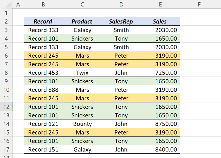
1. Remove Duplicates button
- Select the data → Data → Remove Duplicates.
- Tick My data has headers.
- Tick the columns that together define a duplicate. All columns = only identical rows are removed. Click OK.
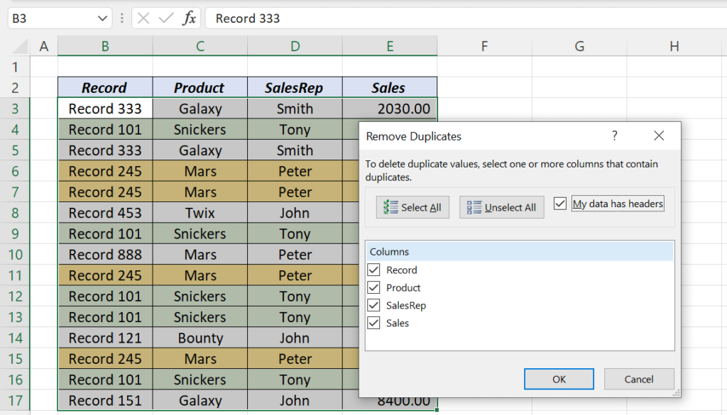
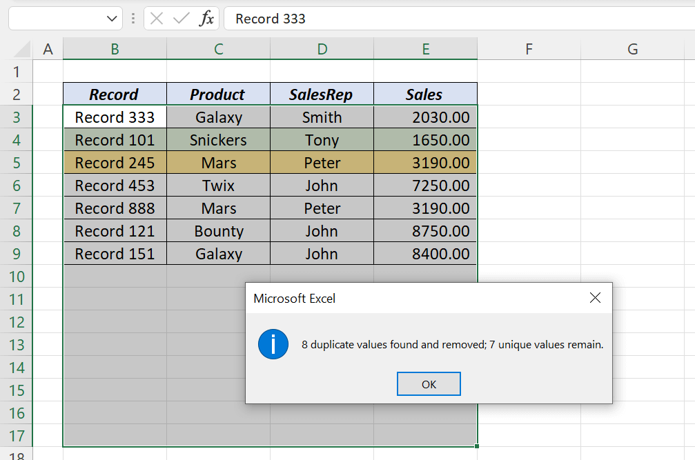
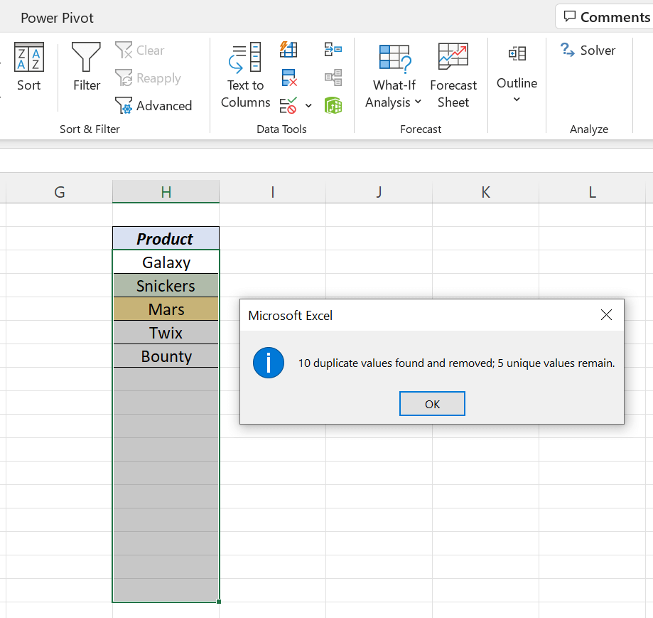
It keeps the first occurrence and deletes the rest. To get a unique list from one column, copy that column elsewhere first and run it there.
2. Advanced Filter
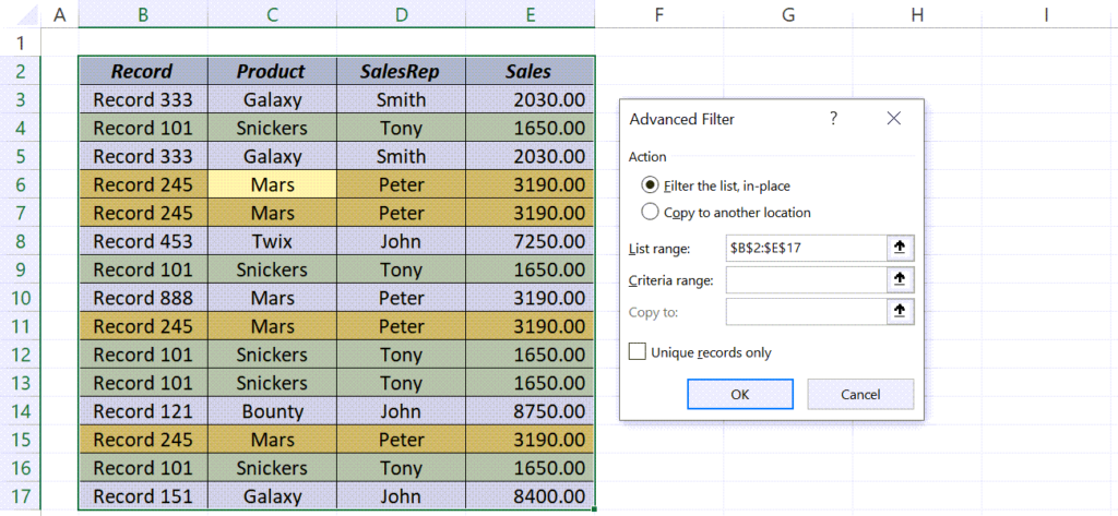
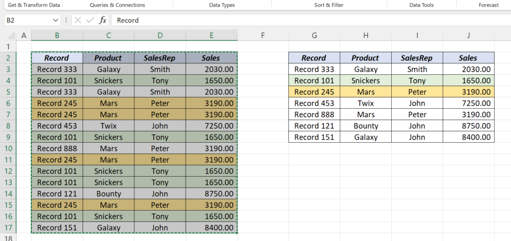
Data → Advanced, choose Copy to another location, set Copy to (such as G2), tick Unique records only, and click OK. The original stays untouched.
3. UNIQUE function (Excel 365)
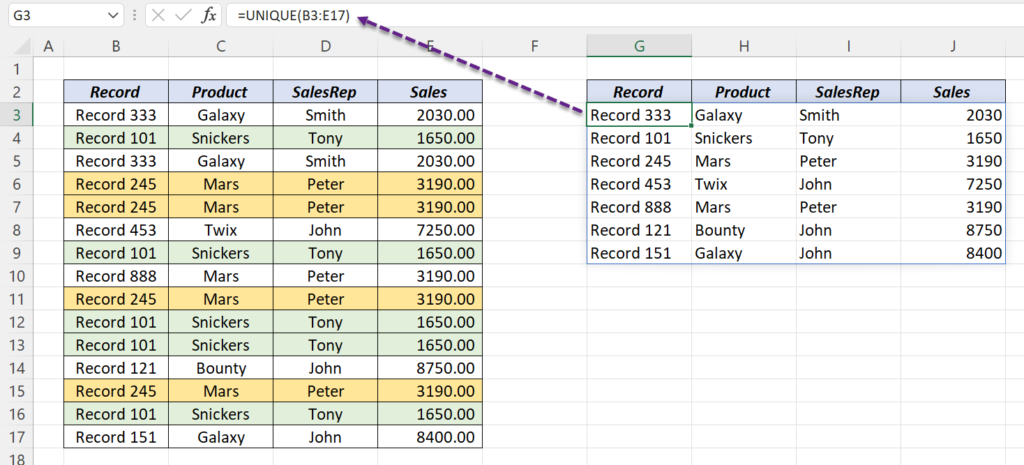
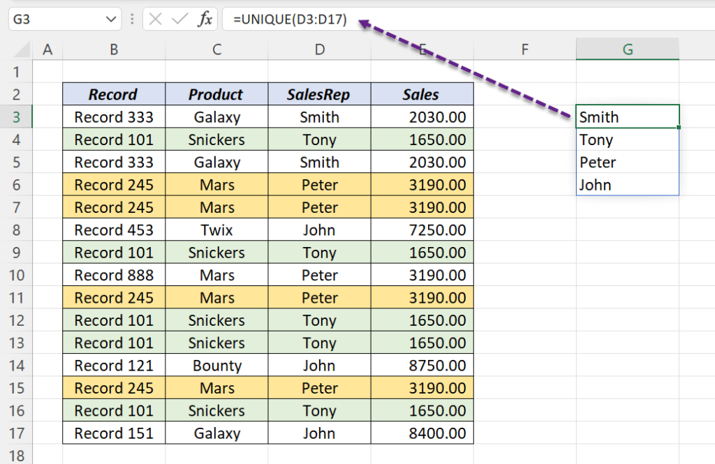
=UNIQUE(B3:E17)Returns the unique rows, and updates as the data changes. One column: =UNIQUE(D3:D17). Sorted: =SORT(UNIQUE(D3:D17)). Values that appear only once: =UNIQUE(D3:D17,,TRUE).
4. COUNTIF helper column
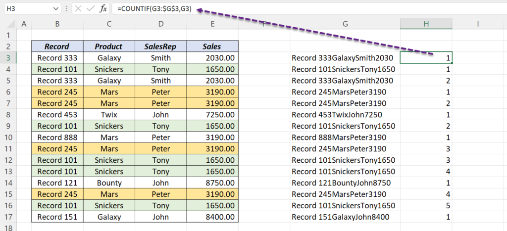
Join each row into one value, then count how many times that combination has appeared so far:
=COUNTIF($F$3:F3,F3)with =TEXTJOIN("|",,B3:E3) in column F. Filter the helper column for values greater than 1 and delete those rows. The | separator stops AB + C matching A + BC.
5. Macro: unique copy on a new sheet
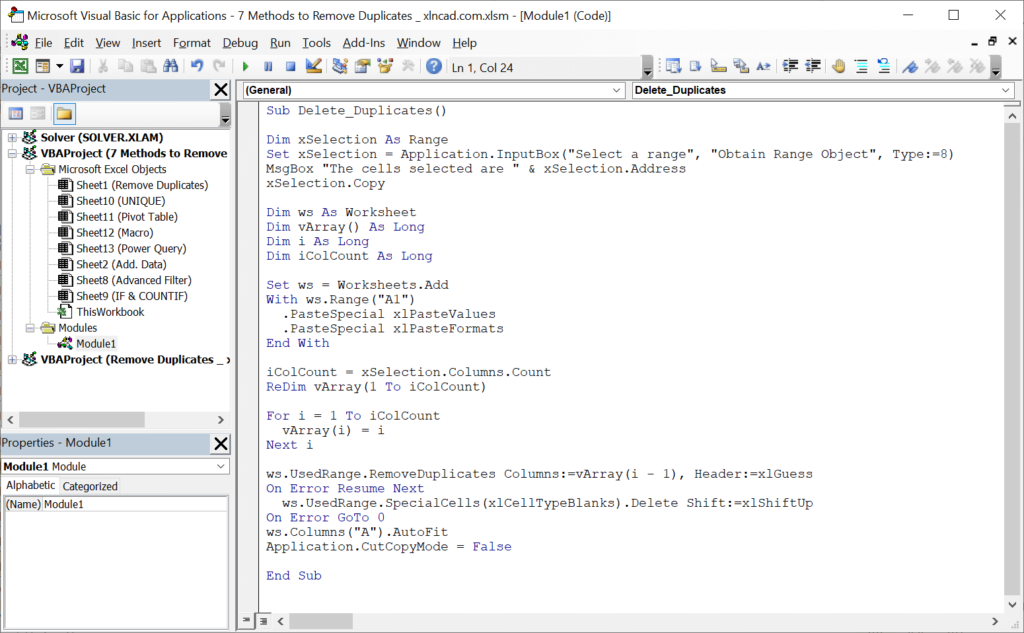
Select the data, including headers, and run:
Sub RemoveDuplicatesToNewSheet()
    Dim r As Range, ws As Worksheet, cols() As Variant, i As Long
    Set r = Selection
    Set ws = Worksheets.Add
    r.Copy ws.Range("A1")
    ReDim cols(0 To r.Columns.Count - 1)
    For i = 0 To UBound(cols): cols(i) = i + 1: Next i
    ws.UsedRange.RemoveDuplicates Columns:=(cols), Header:=xlYes
End SubThe original macro passed only the last column to RemoveDuplicates, so rows that differed in other columns could be deleted. This version checks every column. The brackets around (cols) are required.
6. Power Query (refreshable)
- Click in the data → Data → From Table/Range.
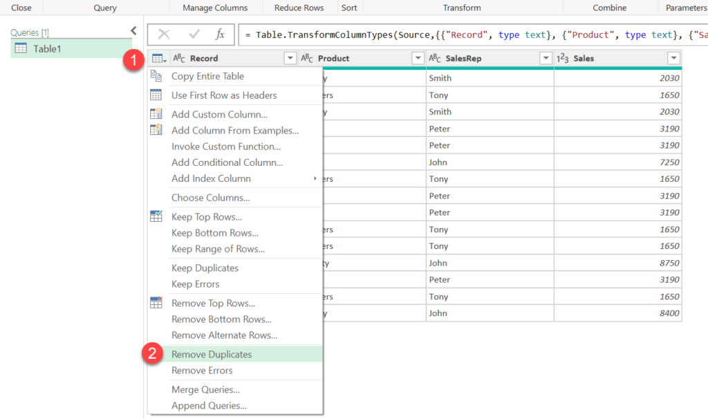
- Select the columns that define a duplicate (or click the table icon at the top-left of the grid for all columns) → right-click → Remove Duplicates.
- Home → Close & Load To.
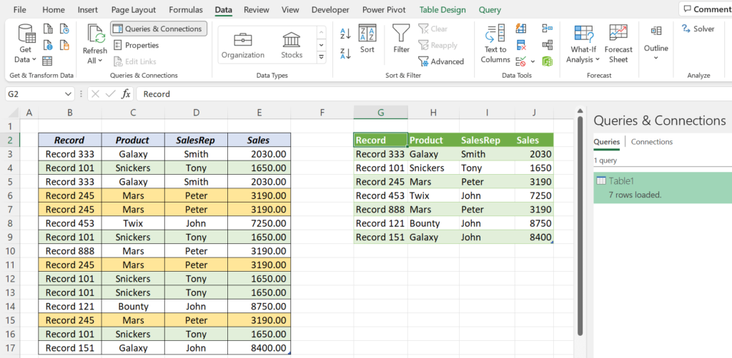
When new rows are added, click Data → Refresh All: no need to repeat the steps. This is the best choice for data you receive every week.
Power Query compares text case-sensitively (Apple and apple are different), unlike the Remove Duplicates button. Add Transform → Format → lowercase first if case shouldn't matter.
7. PivotTable
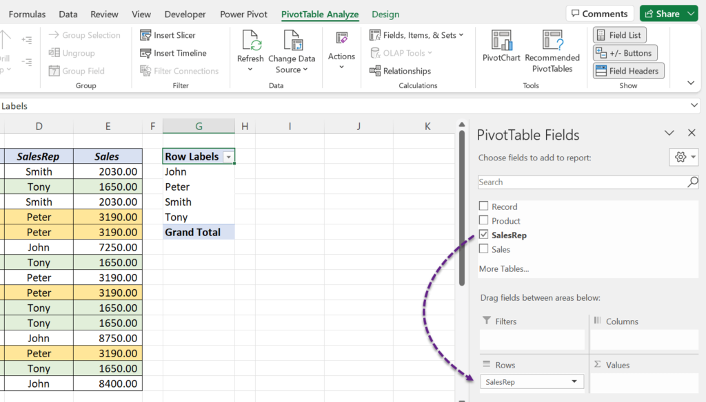
Insert → PivotTable, then drag a field such as SalesRep to Rows. The PivotTable lists each value once. Refresh it when the data changes.
Before you remove anything
- Make a copy, or use a method that doesn't change the original.
- Trim extra spaces first (
=TRIM(B3)), orAjayandAjay(with a space) won't count as duplicates. - To see the duplicates before deleting, use find duplicates. For a quick online clean-up, try the remove duplicates tool.