Following are 3 different methods to find the duplicates in a dataset.
Table of Contents
FILTER Function to find Duplicates
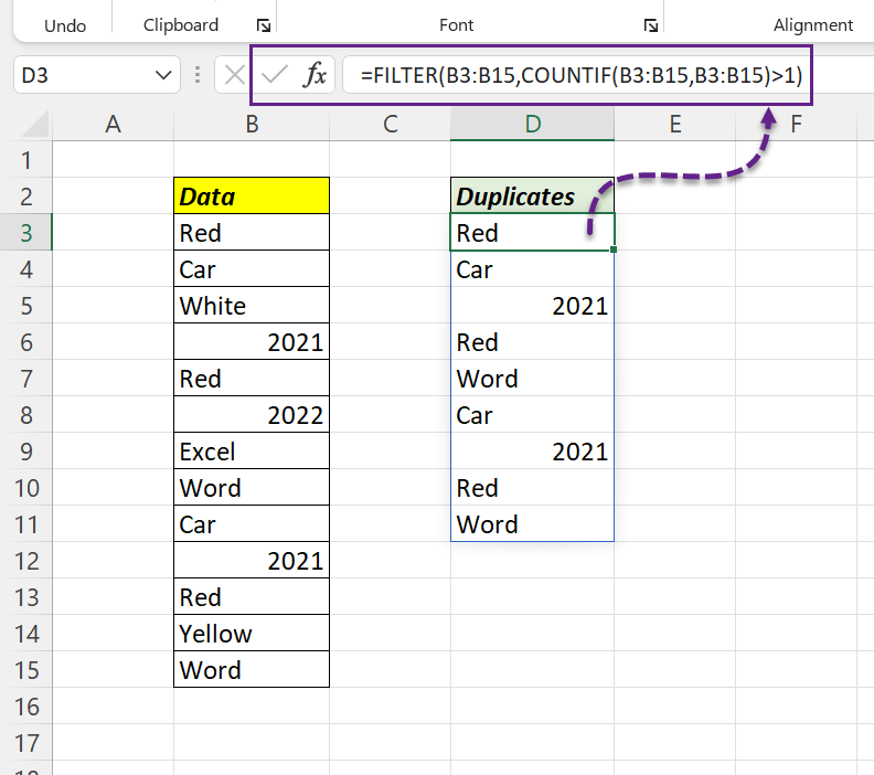
In this formula, we will use the COUNTIF function to find out how many times each value is repeated. Then the FILTER function is used filter out those values with a count greater than 1.
Combining FILTER and COUNTIF function to return the duplicate values in the data range B3:B15
=FILTER(B3:B15,COUNTIF(B3:B15,B3:B15)>1)
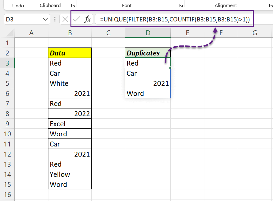
If you want to remove the duplicates from duplicates, wrap the above formula with the UNIQUE function
=UNIQUE(FILTER(B3:B15,COUNTIF(B3:B15,B3:B15)>1))
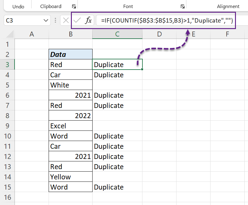
IF and COUNTIF Function to spot the duplicates
Like what we did in the above formula, here also we will use the COUNTIF function to find out how many times each value is repeated in the dataset. Then the IF function is used to check whether the ‘count’ is greater than 1 or not. Greater than 1 means, ‘Duplicate’.
=IF(COUNTIF($B$3:$B$15,B3)>1,"Duplicate","")
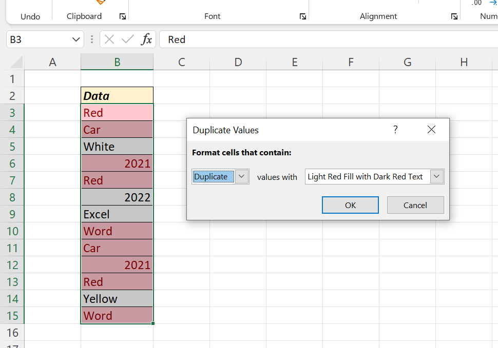
Conditional Formatting to highlight duplicates
Conditional formatting can be used to highlight the Duplicate values as well as the Unique values in a dataset. To highlight the duplicate values, Select the cells containing data > in the Home tab of the Excel Ribbon > Conditional Formatting > Highlight Cells Rules > Duplicate Values…
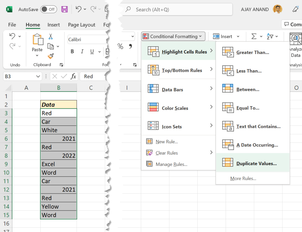
A dialogue called Duplicate Values will be activated, Click on OK and all those Text and Number data with multiple instances will get highlighted.