The Excel UNIQUE function returns the distinct values from a range, removing duplicates. The list updates by itself when the data changes.
array |
The range to take unique values from. |
|---|---|
by_col optional |
FALSE to compare rows (default), TRUE to compare columns. |
exactly_once optional |
TRUE to return only values that appear exactly once. |
Table of Contents
Basic example
To list each region once, give UNIQUE the Region column:
=UNIQUE(B3:B10)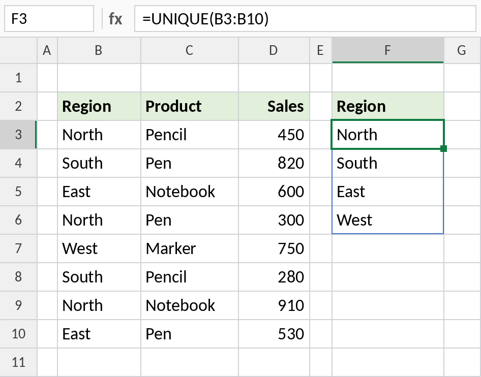
The 8 entries reduce to 4 regions, in the order they first appear: North, South, East, West.
Count unique values
Wrap UNIQUE in COUNTA to count how many distinct values there are:
=COUNTA(UNIQUE(B3:B10))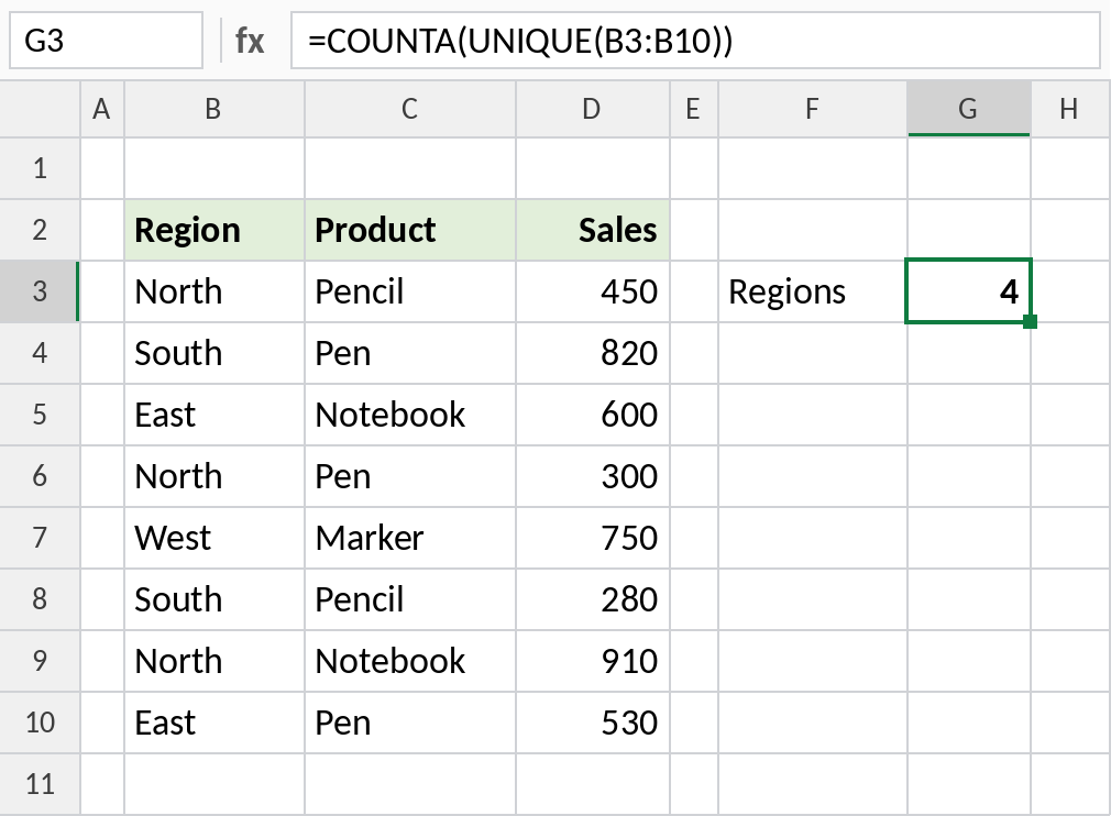
UNIQUE returns 4 regions and COUNTA counts them: 4. This is the simplest way to count distinct items in Excel 365.
Sorted unique list
Wrap UNIQUE in SORT to get the distinct values in alphabetical order:
=SORT(UNIQUE(C3:C10))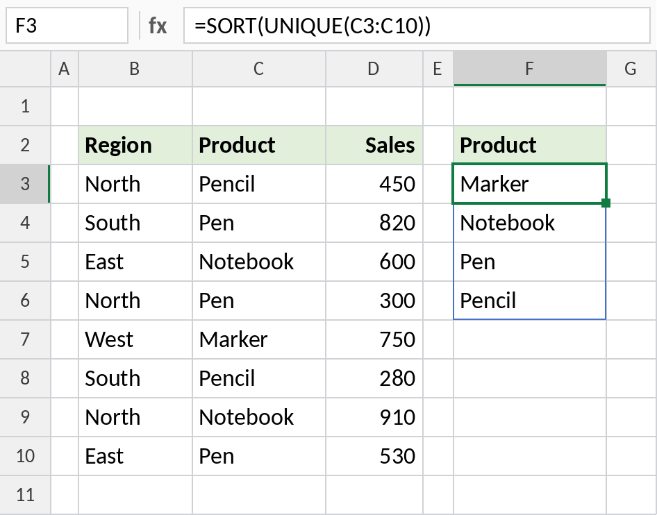
The four products come back A to Z: Marker, Notebook, Pen, Pencil. A sorted unique list makes a good source for a drop-down list.
Values that appear only once
Set the third argument to TRUE to keep only values with no duplicates at all:
=UNIQUE(B3:B10,,TRUE) 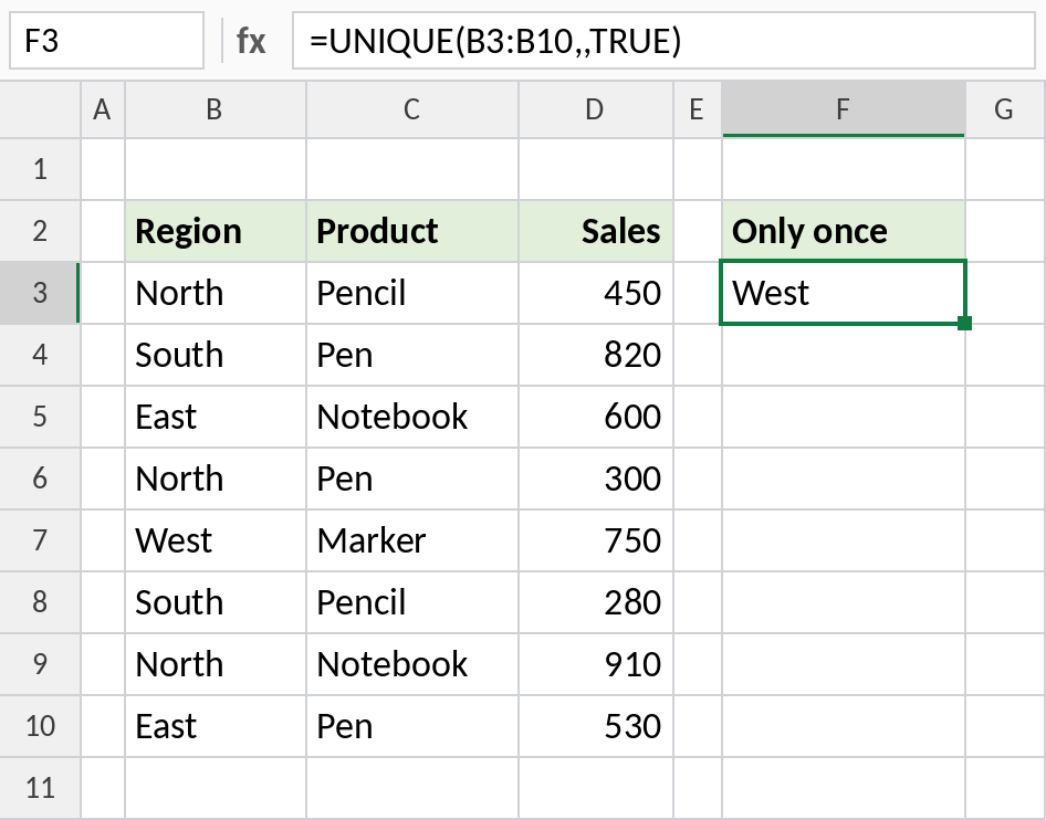
North, South and East each appear more than once, so only West is returned. Note the two commas, which skip the by_col argument.
Remove duplicates: formula vs ribbon
| UNIQUE | Data → Remove Duplicates | |
|---|---|---|
| Changes the original data | No | Yes |
| Updates when data changes | Yes | No, run it again |
| Works in all versions | 2021 and later | All versions |
Notes
- UNIQUE is not case-sensitive: “north” and “North” count as the same value.
- Give it several columns, such as
B3:C10, to get unique combinations of Region and Product. - Blank cells in the range appear in the result as 0. Use
=UNIQUE(FILTER(B3:B20,B3:B20<>""))to skip them. - Keep the spill area empty, or you’ll see
#SPILL!.
Common errors
| Problem | Cause | Fix |
|---|---|---|
#SPILL! |
Cells below the formula aren’t empty | Clear the cells |
| A 0 in the results | The range includes empty cells | Use FILTER to remove blanks first |
| Values that look the same appear twice | Extra spaces, such as “North “ | Clean the data with TRIM |
#NAME? |
Opened in Excel 2019 or earlier | Use Data → Remove Duplicates instead |
Practice file
All four examples with working formulas (Excel 2021 or 365).