Converting data into Excel Table is the best way to keep your data organized. As soon as a data range converted into an Excel Table, it will acquire a set of awesome properties which makes the data easy to handle.
Even if, Excel Tables are available from 2007, this is one of the most underused features of Excel.
If you haven’t used Excel Tables until now, here are 11 Solid Reasons to start using it.
Table of Contents
Excel Tables are easy to Create
To convert a data range into an Excel Table,
Select a cell in the data range and Press CTRL + T. You will get the dialog called Create Table. Click OK and Congrats! Your data is now converted into an Excel Table.
You can also create an Excel Table using the Table button in the Insert tab of the Excel Ribbon
CTRL + L is a lesser known keyboard shortcut to create an Excel Table.
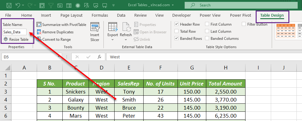
While creating, Excel Tables will be automatically named as Table1, Table2, etc. . But we can rename an Excel Table whenever we want
To rename an Excel Table,
Select the Table > go to the contextual tab called Table Design > Type in the desired name in the input box under the label, Table Name
Note: Excel Table won’t accept spaces in between characters. But we can use underscore ‘_’ instead of space to separate names.
Read about more methods to create an Excel Table
Excel Tables are Dynamic
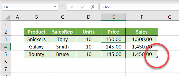
Excel Tables expand, whenever you add additional data into it.
Note the formulas in the following Example. You can see the formulas getting updated automatically, when the Table referred in them are resized.
The small ‘blue handle’ at the bottom right corner of the Excel Table can be used to resize the table.
Note: To make a Drop Down List dynamic, convert the source data into an Excel Table
Note: Due to this dynamic nature, it is always recommended to use Excel Table as source for Pivot Tables.
Excel Tables come with Slicers
Slicers are floating filters which can be used to filter Pivot Tables, Pivot Charts or Excel Tables.
To create Slicers for an Excel Table,
Select the Table > go to the Table Design tab > Click on Insert Slicer > in the dialog for Insert Slicers, mark the check boxes for the columns which you want to create Slicers > Click OK
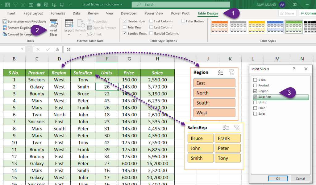
Once you click on the related Slicer, Excel Table will update accordingly.
Excel Tables can create meaningful Formulas
Excel Tables use Structured References instead of normal Cell References. By giving appropriate names to columns of an Excel Table, we can create meaningful, human readable formulas which will be easier to understand.
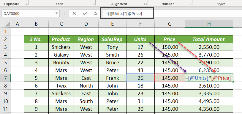
Note the formula in the cell H7 of the following image. If it was a normal data range, the formula would have been =F7*G7
As the data range is an Excel Table,
the formula is displayed as =[@Units]*[@Price], which tells us that value in the column called Units is multiplied by the value in the Column Price.
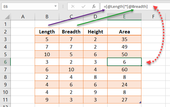
See the following examples, where structured references are used to create meaningful formulas.
The following formula is used in the column called Area to return the area of measurements specified in the columns Length and Breadth.
=[@Length]*[@Breadth]
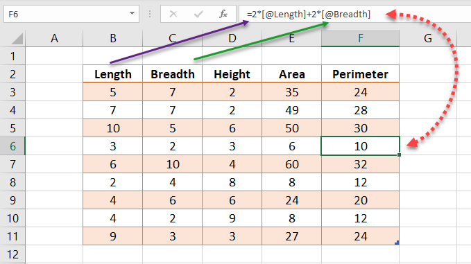
To find the Perimeter,
=2[@Length]+2[@Breadth]
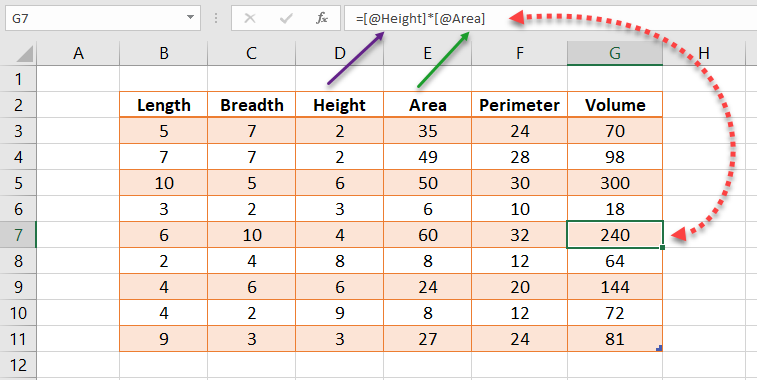
For Volume, third column called Height is multiplied by the fourth column called Area, which contains the values for area
=[@Height]*[@Area]
Automatic Formulas
Excel tables are associated with a feature called Calculated Columns which will apply the same formula to an entire column.
You just need to enter the formula into any cell of a column and that formula will be automatically applied to the entire column.
Note: Any changes made to the formula in a cell which is a part of an Excel Table, will be automatically applied to the entire column.
Total Row
Total Row is another great feature of Excel Tables which will provide aggregations like Average, Count, Sum, etc., of a column without entering a formula.
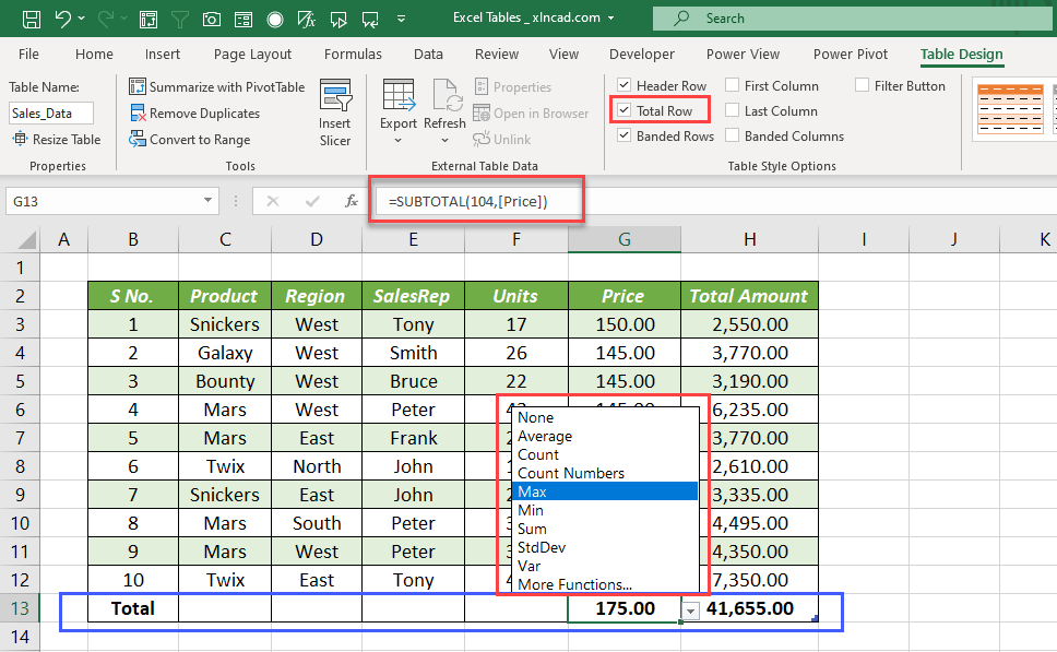
As the Total Row feature is powered with SUBTOTAL function, it will always return the totals from the visible cells of a column.
CTRL + SHIFT + T is keyboard shortcut to Display/Hide the Total Row
We can easily Navigate to Excel Tables
All Excel Tables present in an Excel workbook will be listed in the Excel Name Box.
To navigate to a particular table, click on the drop down arrow with the Excel Name Box and select the table name. You will be taken to the selected table (even if the table is in another worksheet).
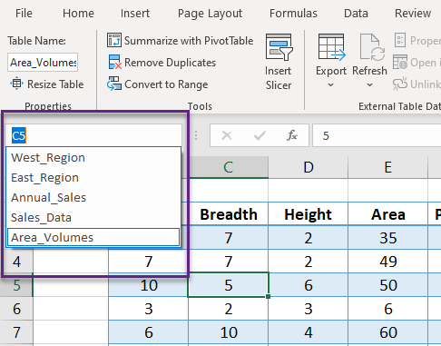
Table headers stays visible
Column Headers of Excel Tables always stay visible while scrolling down through it. Means you don’t need to use the Freeze Panes option.
Excel Tables can be easily formatted
Availability of many predefined formats makes formatting of Tables easy.
To change the Visual Style of an Excel Table,
Select the Table > go to the Table Styles group in the Table Design tab > click on the drop down arrow called More to see the available Table Styles > hover through the formats for the preview of each style and click on a Style to apply it to the Table.
Recover deleted data
When you delete a record using the in built Data Entry Form of Excel, data will be lost beyond recovery.
But, if the data is in the form of an Excel Table, deleted data can be recovered using the Undo option.
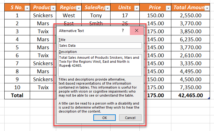
Alternate Text
Like any other object in Excel, Table also have the option to add Alternative Text (Alt Text) to it.
Alt Text helps people with vision or cognitive impairments to understand pictures and other graphical content.
To add Alternative Text to an Excel Table,
Right-click on the Table > Table > Alternative Text
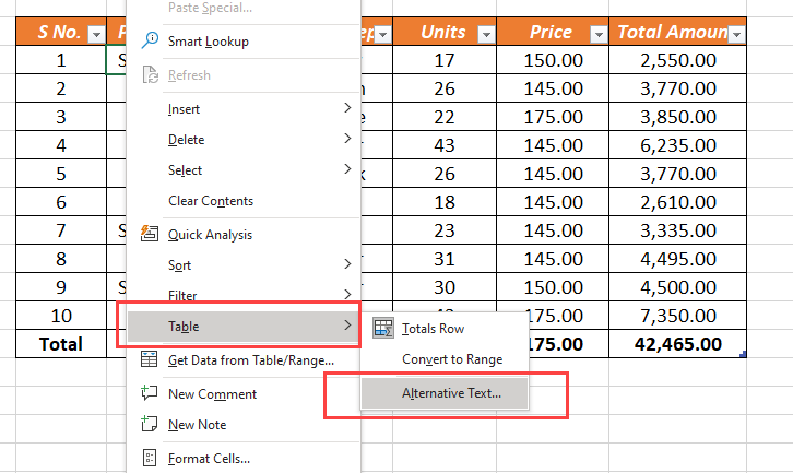
Type in the Title, Description and Click OK
Shortcuts for Excel Tables
| Create Table | CTRL + T |
| Create Table | CTRL + L |
| Select Table | CTRL + A |
| Select Table Row | SHIFT + SPACE |
| Select Table Column | CTRL + SPACE |
| Toggle AutoFilter | CTRL + SHIFT + T |
Different Methods to Create Excel Tables