Sum Colored Cells in Excel: 3 Ways, With and Without VBA

Q: How do I count coloured cells instead of summing them?

Use the same tricks: =SUBTOTAL(103, range) with Filter by Color, read Count in the status bar after Find All, or change the VBA line to add 1 instead of the value.

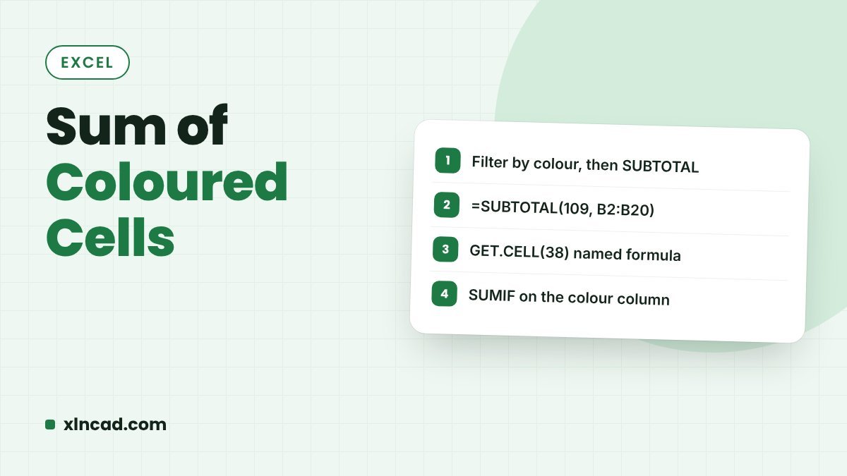
Excel has no built-in function that reads cell colour, but you can get the sum of coloured cells in three ways: filter by colour and use =SUBTOTAL(109, range), select the coloured cells with Find & Select and read the sum from the status bar, or write a small VBA function. If the colour comes from a rule, such as “amount over 500”, sum by the rule itself with SUMIF instead.

Quickest wayFilter by colour + SUBTOTAL(109)

One-off checkFind & Select by format, read the status bar

Reusable formulaA short VBA function (SumByColor)

Conditional formattingSum by the rule, not the colour

Watch the short video: sum of values in coloured cells

Method 1: Filter by colour and SUBTOTAL

In a cell above or below the data, enter =SUBTOTAL(109, B2:B20). 109 means SUM, ignoring rows hidden by the filter.
Turn on the filter with Ctrl + Shift + L.
Open the filter arrow, choose Filter by Color and pick the colour.

The SUBTOTAL result now shows the sum of only the visible, coloured rows. Pick another colour and it updates at once.

Method 2: Find & Select, then read the status bar

Press Ctrl + F, click Options, then Format, and pick the fill colour on the Fill tab. You can also use Choose Format From Cell to pick it up from the sheet.
Click Find All, then press Ctrl + A inside the results list.

Every cell with that colour is now selected, and the status bar at the bottom shows their Sum, Average and Count. Nothing is written to the sheet, which makes this the fastest one-off check. The same dialog can also replace a cell colour.

Method 3: A small VBA function

For a live formula in the sheet, add this function. Press Alt + F11, go to Insert > Module and paste:

Function SumByColor(rng As Range, ref As Range) As Double
  Dim c As Range
  For Each c In rng
    If c.Interior.Color = ref.Interior.Color Then
      SumByColor = SumByColor + c.Value
    End If
  Next c
End Function

Colour one spare cell, say D2, with the colour you want to total.
Enter =SumByColor(B2:B20, D2).
Save the workbook as .xlsm (macro-enabled), or the function is lost when you close it.

Changing a cell’s colour does not trigger a recalculation, so after recolouring press Ctrl + Alt + F9 to refresh the result.

What about conditional formatting colours?

None of these methods see colours applied by conditional formatting: the filter works, but GET.CELL and Interior.Color read the manually applied colour, not the displayed one. Since a conditional colour always comes from a rule, sum by the rule itself: if cells turn red when the value is over 500, use =SUMIF(B2:B20, ">500").

Frequently asked questions

Can SUMIF sum by colour directly?

No. SUMIF tests values, not formatting, and no built-in Excel function reads cell colour. Use the filter, the status bar or the VBA function above.

How do I count coloured cells instead of summing them?

Use the same tricks: =SUBTOTAL(103, range) with Filter by Color, read Count in the status bar after Find All, or change the VBA line to add 1 instead of the value.

Why does the VBA result not update when I recolour cells?

Recolouring does not trigger recalculation. Press Ctrl + Alt + F9 to force a full recalculation after changing colours.

Does this work in Google Sheets?

Not with these exact tools. In Google Sheets, filter by colour and use SUBTOTAL(109, range), or sum by the rule behind the colour.

How to Sum Colored Cells in Excel (3 Methods)