
Power Query's Group By turns a long list of transactions into a summary: total sales per product, count of orders per region, or several totals at once. Unlike a formula summary, it refreshes with one click when new rows arrive.
The data
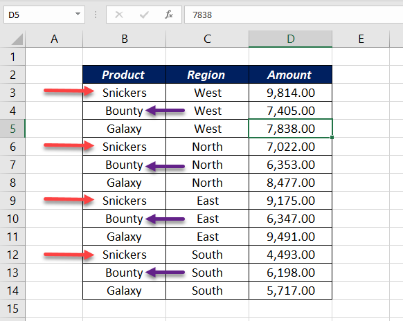
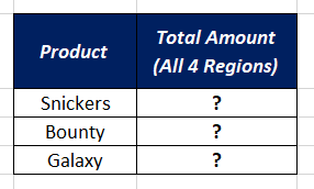
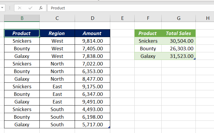
Sales of Snickers, Bounty and Galaxy across four regions. The goal is total sales for each product.
Step 1: Load the data
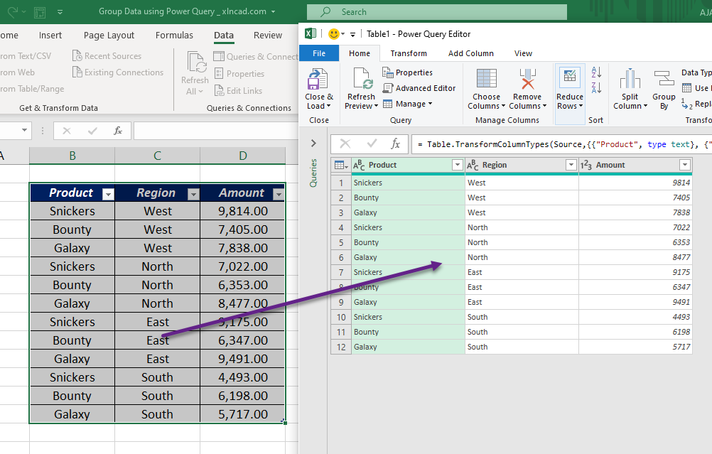
Click in the data → Data → From Table/Range → OK.
Step 2: Group By
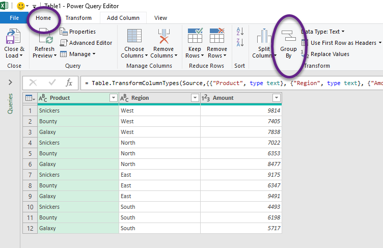
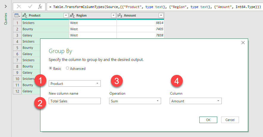
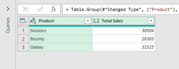
Home → Group By. In the dialog, choose the column to group by (Product), a name for the new column (Total Sales), the operation (Sum) and the column to total (Amount).
Step 3: Load and refresh
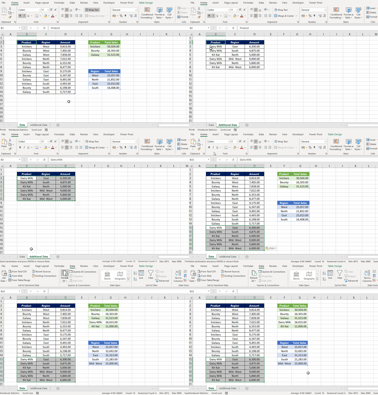
Home → Close & Load To → Existing worksheet. When the source changes, click Data → Refresh All.
Advanced: several columns and totals
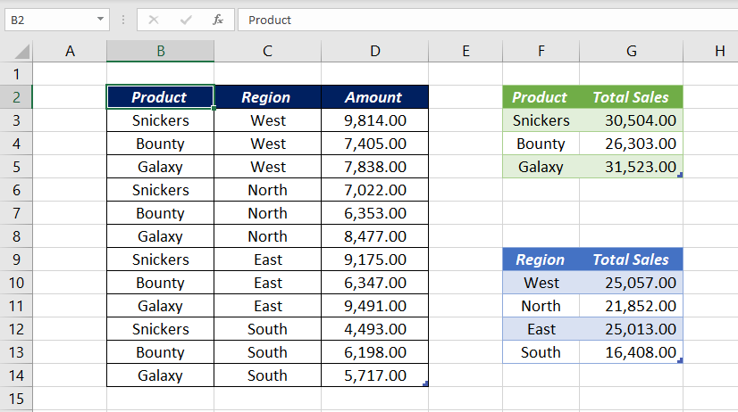
Choose Advanced in the Group By dialog to group by more than one column, such as Region and Product, and click Add aggregation for more results in one step:
| New column | Operation | Column |
|---|---|---|
| Total Sales | Sum | Amount |
| Orders | Count Rows | (none) |
| Average Sale | Average | Amount |
| Largest Sale | Max | Amount |
Count Distinct Rows counts unique combinations, and All Rows keeps each group's rows as a nested table, useful for numbering within groups or picking the top item per group.
Formula alternative (Excel 365)
=GROUPBY(Sales[Product],Sales[Amount],SUM)GROUPBY gives the same summary as a live formula, with no refresh needed. Use Power Query when the data comes from other files or needs cleaning first.