We can use either the TRANSPOSE function or the Paste Special Transpose option to transpose data in Excel.
Here is one more method to transpose data, which is using the Power Query in Excel.
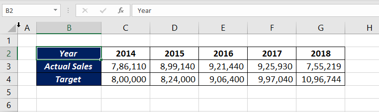
Following is the data which is I want to Transpose.
To transpose this data using Power Query,
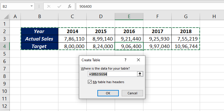
Select a cell in the data set > Click on From Table/Range > Click OK in the Create Table Dialog
Selected data is loaded in the Power Query Editor.
Also note that the first row of the data set has become the column headers.
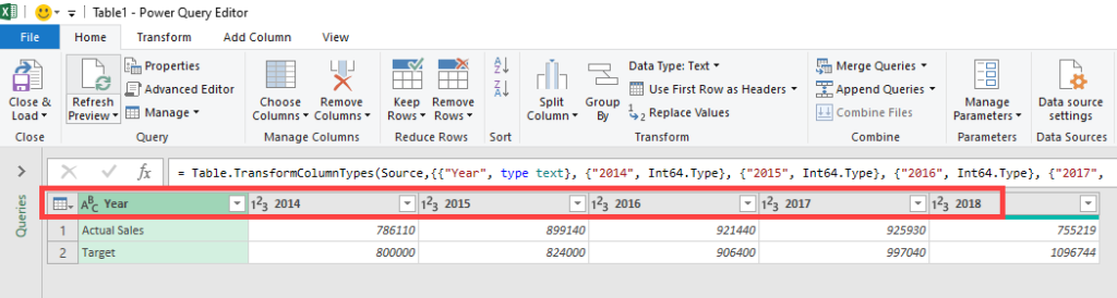
Before using the Transpose option of Power Query we should demote these column headers as the first row.
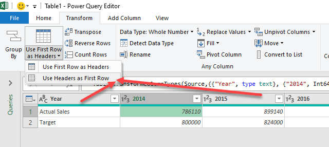
In the Transform Tab > click on Use Headers as First Row
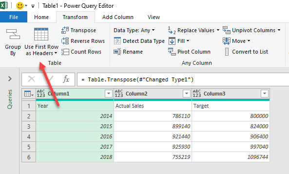
Now that the column headers came down to the first row, click on Transpose in the Transpose Tab of the Power Query Editor
The rows have become the columns and columns have become the rows. Before loading this data into the Excel worksheet, we have to promote the first row as Headers.
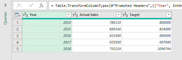
For that, click on Use First Row as Headers in the Transform Tab.
Now the data is the required format and ready to get loaded into a worksheet.
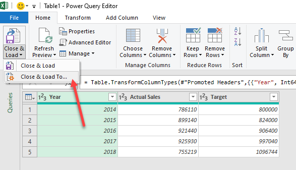
To load this data into an Excel worksheet > Home tab > Close & Load > Close & Load to
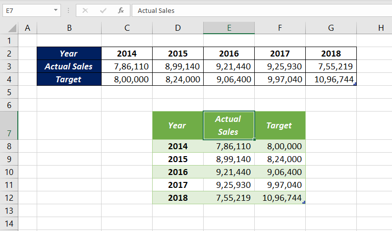
In the Import Data dialog, select Existing worksheet > select the cell where you want to place the transformed table (Here, I have selected the cell D7) and Click OK
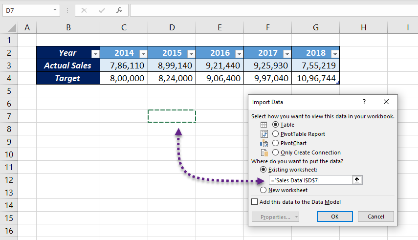
In the data range from D7 to F12, we have the transposed form of data in B2:G4.
Whenever you add something to the source table, right-click on the output table and select Refresh to update it.