To see how many times each item appears, use UNIQUE and COUNTIF in Excel 365, GROUPBY for a sorted summary, a PivotTable, or Power Query’s Group By. All four update when the list changes.
Table of Contents
The list
The list is an Excel Table named ABCD with one column, Items.

1. UNIQUE and COUNTIF (Excel 365)
=HSTACK(UNIQUE(ABCD[Items]),COUNTIF(ABCD[Items],UNIQUE(ABCD[Items])))UNIQUE lists each item once; COUNTIF counts each one. HSTACK puts them in two columns side by side.


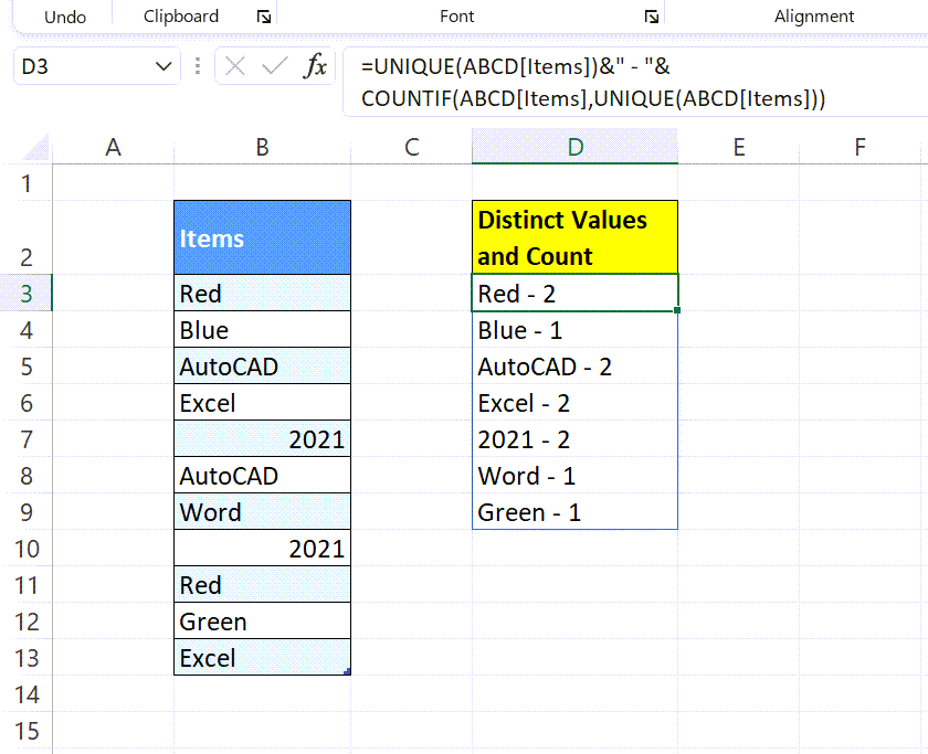
For one column of text such as Apple – 4: =UNIQUE(ABCD[Items])&" - "&COUNTIF(ABCD[Items],UNIQUE(ABCD[Items])).
2. GROUPBY (current Excel 365)
=GROUPBY(ABCD[Items],ABCD[Items],COUNTA,0,0,-2)Returns each item with its count, sorted from most to least. See GROUPBY.
3. PivotTable
Select the table → Table Design → Summarize with PivotTable → OK. Drag Items to Rows and again to Values.


Right-click → Refresh after the list changes.
4. Power Query
Data → From Table/Range → Home → Group By → Count Rows → OK → Close & Load To.


All four updating
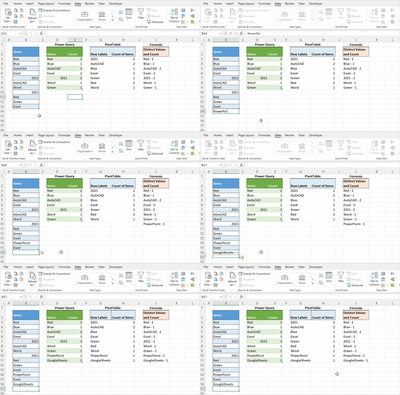
Formulas update instantly; the PivotTable and Power Query update when you click Refresh.