Every Excel error code tells you what went wrong: #DIV/0! is a division by zero, #N/A is a value that wasn’t found, #REF! is a reference that no longer exists. Here is what each error means, a typical cause, and how to fix it.
Table of Contents
Quick reference
| Error | Means | Usual fix |
|---|---|---|
#DIV/0! |
Dividing by zero or an empty cell | Check the divisor, or =IF(D5=0,"",C5/D5) |
#N/A |
A lookup value wasn’t found | Check spelling and spaces; use XLOOKUP’s if_not_found or IFNA |
#NAME? |
Excel doesn’t recognise a name | Fix the function or range name; add quotes around text |
#VALUE! |
Wrong type of value, such as text in a sum | Find the text cell; convert with VALUE |
#REF! |
A referenced cell was deleted | Undo, or rebuild the reference |
#NUM! |
A number is impossible or too large | Check the inputs, such as negative square roots |
#NULL! |
A space between two ranges that don’t overlap | Use a comma or colon instead |
#SPILL! |
A spill range is blocked | Clear the cells in the way |
#CALC! |
The result is an empty array | Add an if_empty value, such as in FILTER |
#FIELD! |
The field doesn’t exist for that data type | Use a valid field name |
#BUSY! / #CONNECT! |
Data is still loading / no connection | Wait, or check the internet connection |
##### |
Column too narrow (not an error) | Widen the column |
#DIV/0! — division by zero
Excel treats an empty cell as zero, so =C5/D5 returns #DIV/0! when D5 is blank or 0. AVERAGE of a range with no numbers gives the same error.
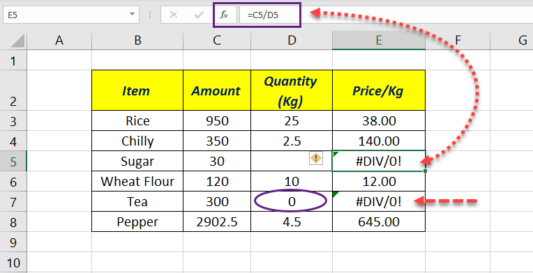
Fix: check the divisor first: =IF(D5=0,"",C5/D5). Avoid hiding it with IFERROR, which also hides other mistakes.
#N/A — value not available
Lookup functions such as VLOOKUP, XLOOKUP and MATCH return #N/A when they can’t find the lookup value.
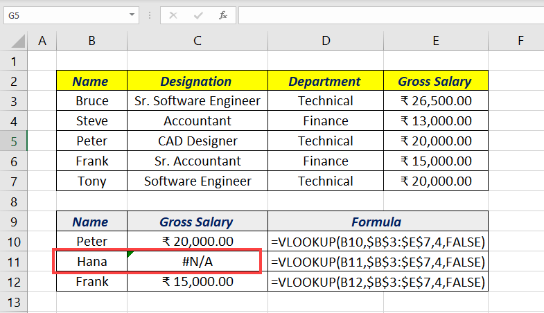
Fix: check for extra spaces (TRIM), numbers stored as text, or a lookup range that doesn’t include the value. To show a message instead, use =XLOOKUP(A2,B:B,C:C,"Not found") or =IFNA(VLOOKUP(...),"Not found"). See VLOOKUP from two tables.
#NAME? — Excel doesn’t recognise a name
A misspelled function (=SU(A1:A5)), a named range that doesn’t exist, or text without quotation marks (=IF(A1=Yes,...)) all give #NAME?. So does a newer function, such as XLOOKUP, opened in an older Excel version.
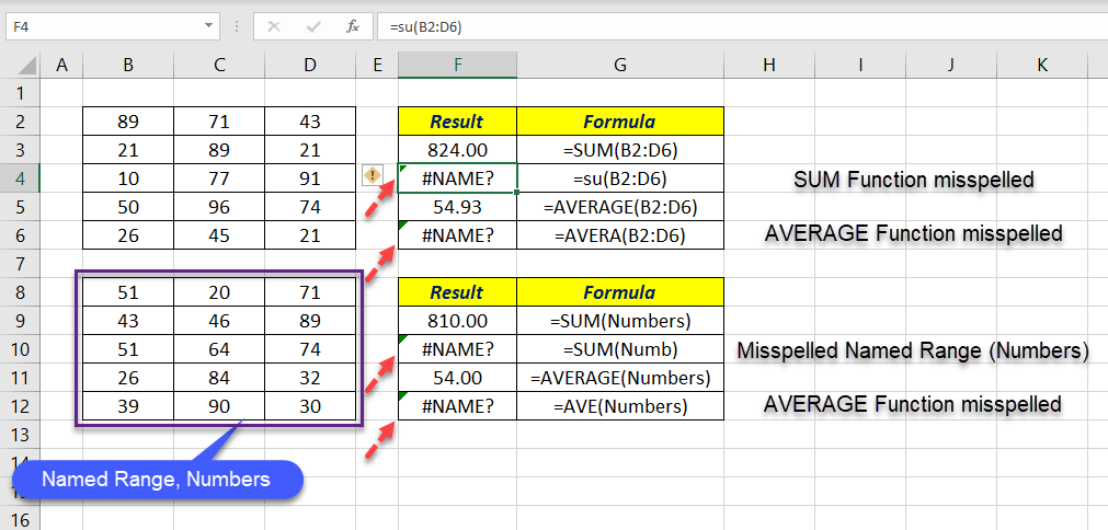
Fix: start typing the function and pick it from the list; check Formulas → Name Manager; put text inside “quotes”.
#VALUE! — wrong type of value
Using text where a number or date is expected, such as ="abc"*5, or a date stored as text in a date function.
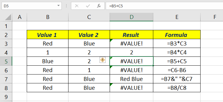
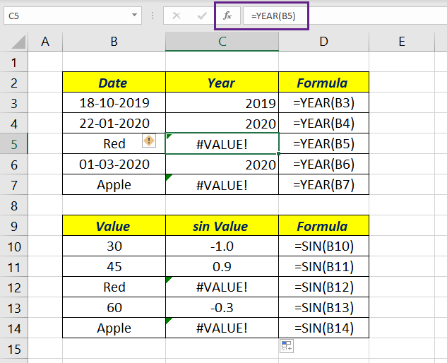
Fix: find the text value. A cell that looks blank may contain a space. Use SUM instead of +, because SUM ignores text: =SUM(A1:A3) works where =A1+A2+A3 fails.
#REF! — invalid reference
A formula pointed to a cell, row, column or sheet that was deleted, or was copied to a place where its relative references would fall off the sheet.
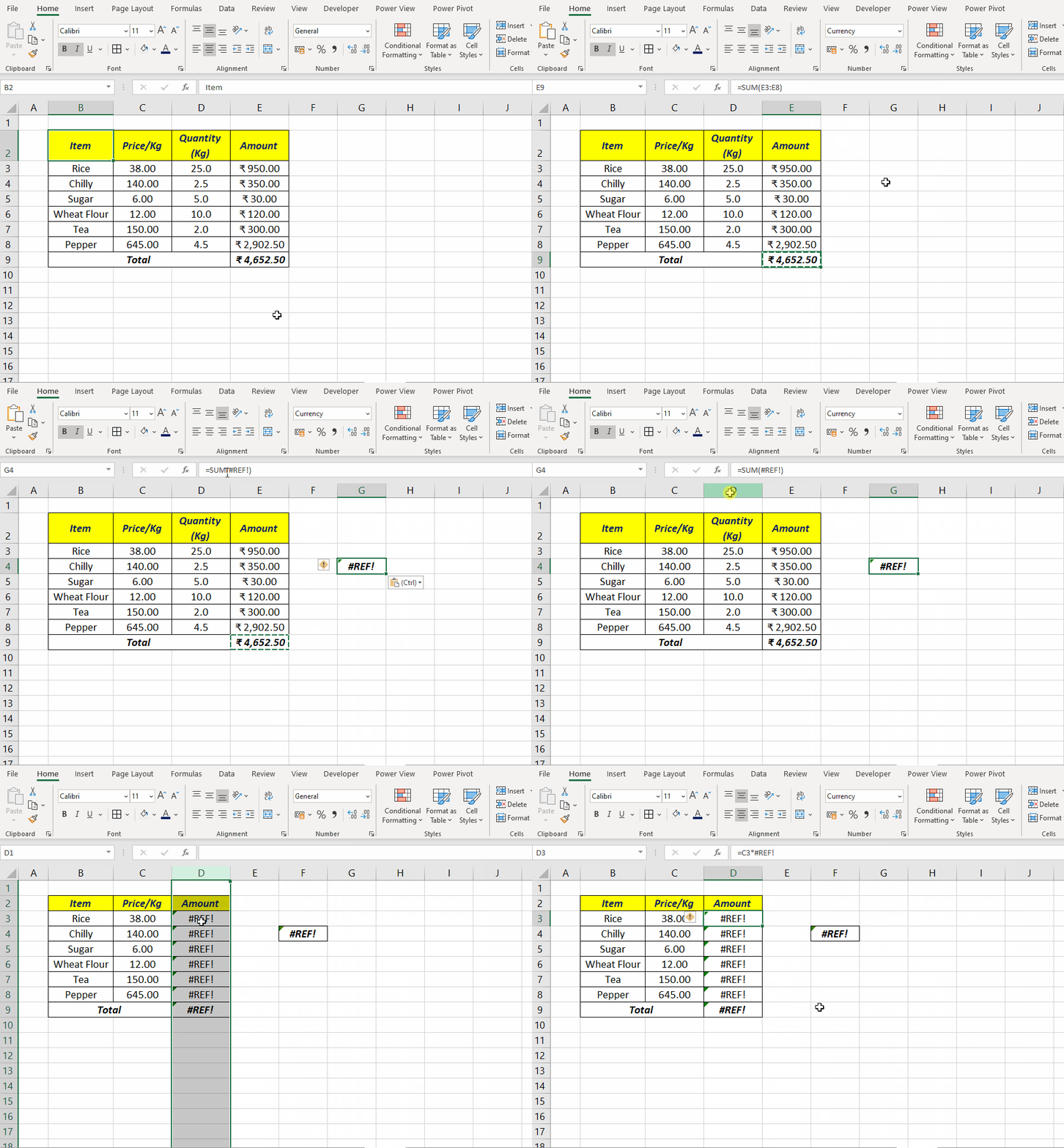
Fix: press Ctrl + Z straight away. Once the file is saved, the original reference is gone, and you’ll need to rebuild the formula. Excel Tables and XLOOKUP are less likely to break when columns are deleted.
#NUM! — invalid number
An impossible calculation, such as =SQRT(-25), a result too large for Excel (above about 1.8 × 10^308), or a function that can’t find an answer, such as IRR. DATEDIF returns #NUM! if the start date is after the end date.
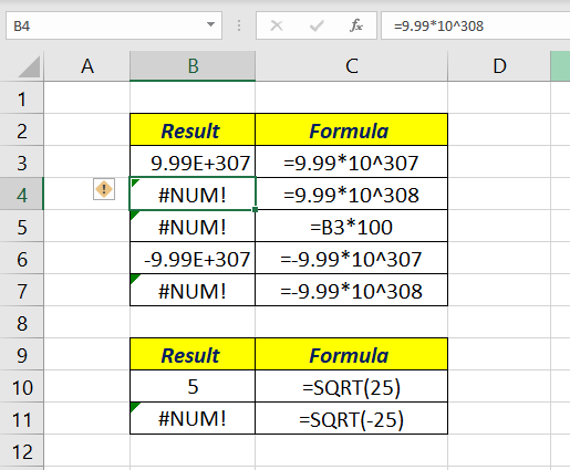
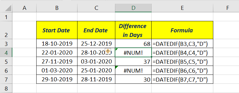
Fix: check the inputs are in the valid range and in the right order.
#NULL! — ranges that don’t meet
A space between two references is Excel’s intersection operator: it returns the cell where they overlap. =SUM(B3 B8) has no overlap, so it returns #NULL!.
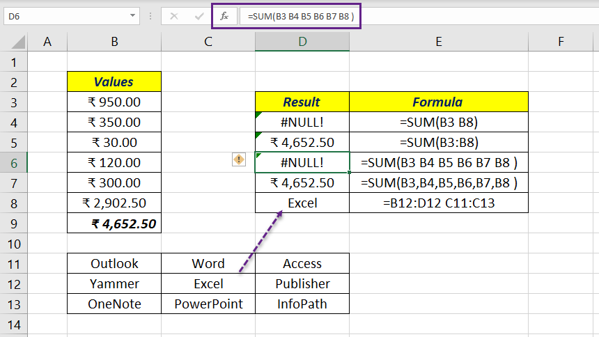
Fix: use a comma for separate cells (=SUM(B3,B8)) or a colon for a range (=SUM(B3:B8)).
##### — column too narrow
Not an error: the number or date is wider than the column. It also appears for negative dates and times.
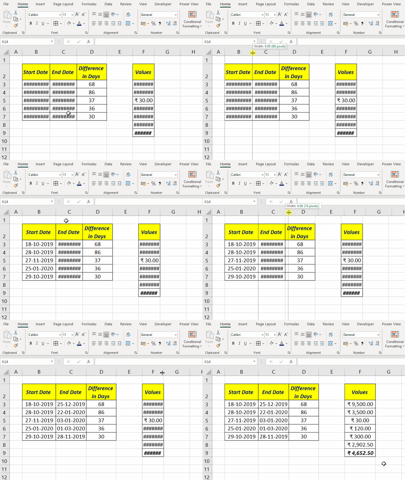
Fix: double-click the column border to AutoFit.
#SPILL! — spill range blocked
A dynamic array formula, such as UNIQUE or FILTER, needs empty cells to spill into. Anything in the way, even a space, blocks it.
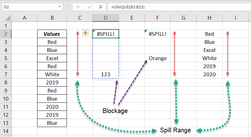
Fix: click the error, then the warning icon → Select Obstructing Cells, and clear them. Spills also can’t go into an Excel Table or merged cells.
#CALC! — empty result
Most often, FILTER finds no matching rows and has nothing to return.
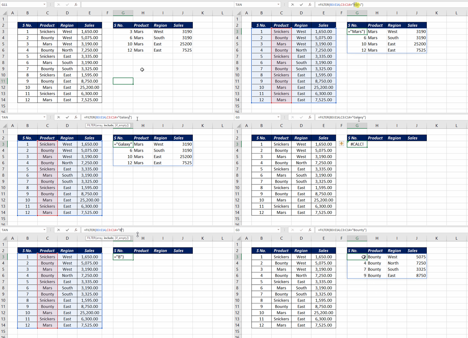
Fix: give FILTER a third argument: =FILTER(A2:C20,B2:B20="Galaxy","No match").
#FIELD! — field not found
With linked data types such as Stocks and Geography, =B6.Capital works for a country but =B7.Capital fails for a stock, because stocks have no capital.
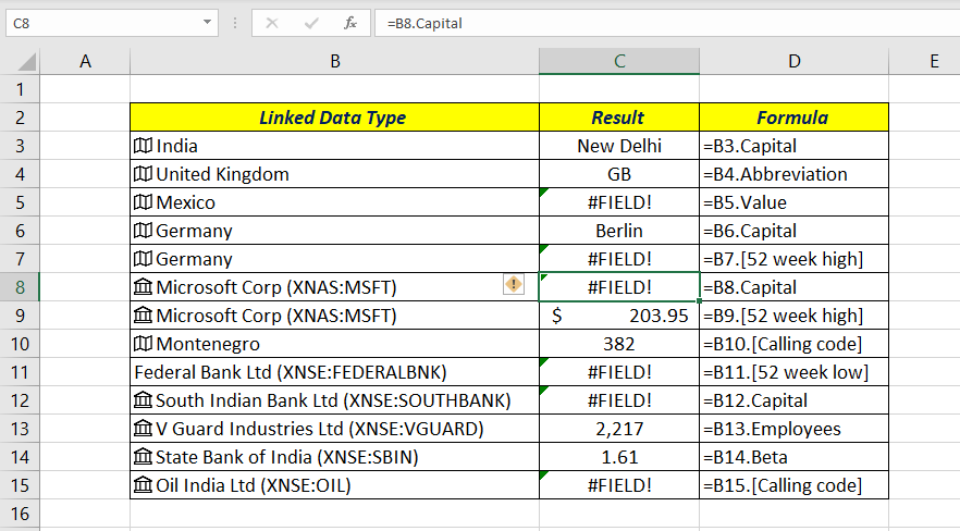
Fix: click the data-type icon to see which fields are available.
#BUSY!, #CONNECT! and #BLOCKED!
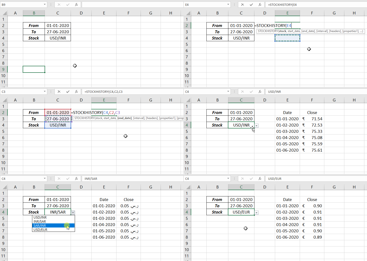
These come from functions that fetch online data, such as STOCKHISTORY. #BUSY! means Excel is still loading and usually disappears in a moment. #CONNECT! means it couldn’t reach the service. #BLOCKED! means the feature or data access is turned off, often by an organization’s settings.
Tools for finding and fixing errors
| Tool | Where | Use it to |
|---|---|---|
| Error Checking | Click the green triangle or Formulas → Error Checking | See why Excel flags a cell |
| Trace Error | Formulas → Error Checking → Trace Error | Draw arrows to the cell causing the error |
| Evaluate Formula | Formulas → Evaluate Formula | Step through the calculation one part at a time |
| Go To Special | Ctrl + G → Special → Formulas → Errors | Select every error cell at once |
| Count errors | =SUMPRODUCT(--ISERROR(A1:D100)) |
Count cells that contain errors |
| Ignore errors in a total | =AGGREGATE(9,6,A1:A100) |
Sum while skipping errors |
IFERROR or IFNA? IFERROR hides every error, including typing mistakes you’d want to see. Use IFNA when you only expect not found.
Frequently asked questions
Why does my VLOOKUP return #N/A when the value is there?
Usually an extra space, or a number stored as text in one list and as a number in the other. Wrap the lookup value in TRIM, or convert both to the same type.
How do I hide all errors when printing?
Page Layout → Page Setup dialog → Sheet tab → Cell errors as → blank.