The VLOOKUP function in Excel is designed to search for a ‘Lookup Value’ in the first column of the specified Table and return the corresponding Value against the first matching Value.
But what if there are two tables, one of which has the possible matching value?
A single VLOOKUP function can’t lookup into two different Tables. We have to combine VLOOKUP with another function in Excel for this purpose.
This is blog post is about a performing VLOOKUP from multiple Tables in Excel.
Following is the weekly Sales data of a distribution company which deals with different Chocolates brands. Each record in the table below contains the Product Code of a Chocolate brand and number of boxes of that brand sold by each Sales person.
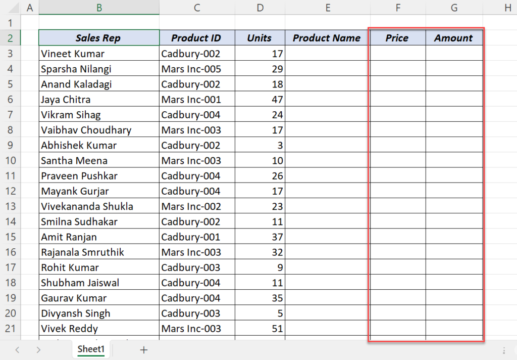
Calculate Total Sales
To calculate the Sales done by each person and the Total Sales Amount, we need the Price of each Product.
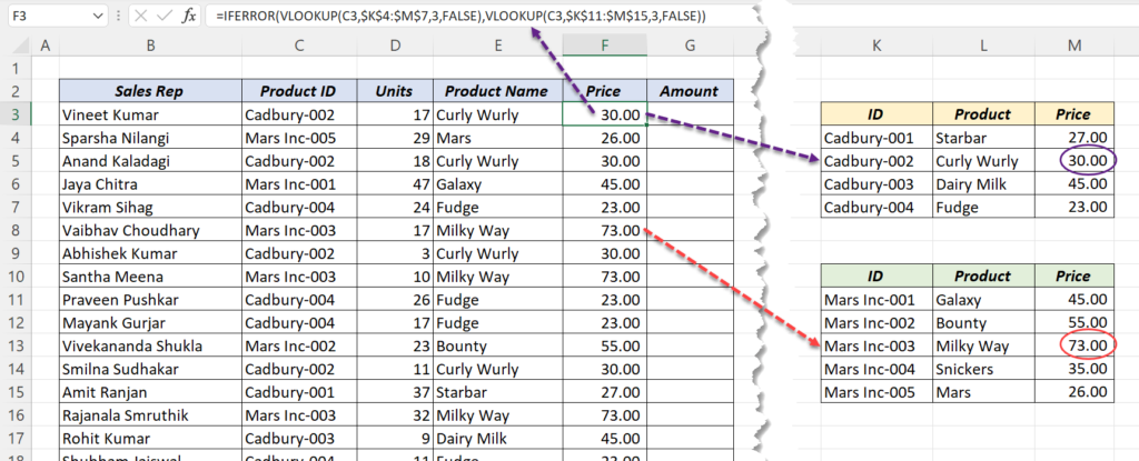
As our distributor is dealing with two companies Cadbury and Mars, the Name and Price of the Products are in two different tables.
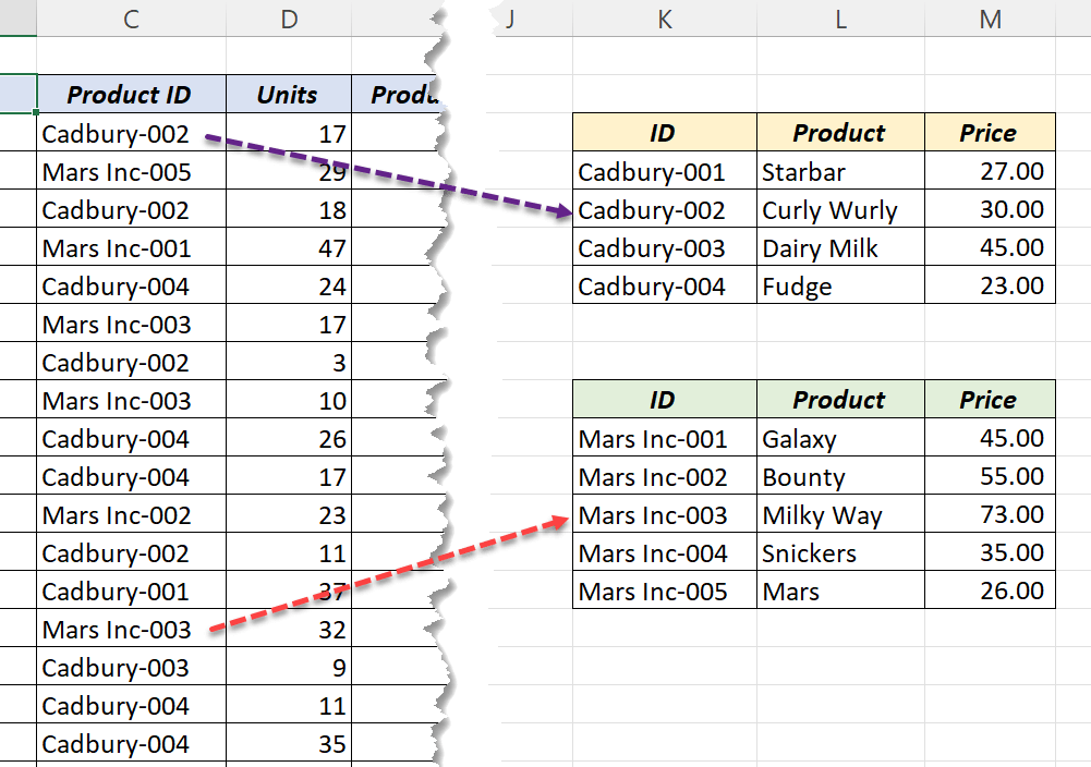
So, we need to find the Product Prices from two different tables using the corresponding Product Codes.
A single VLOOKUP function can extract the Product Name and Price from any one of the two tables, either Cadbury or Mars.
If we use VLOOKUP formula to lookup into the table containing Products of Cadbury, the formula will return #N/A error for the Product Codes of Mars.
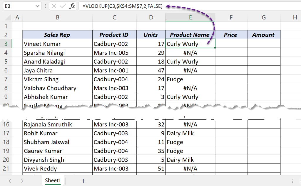
Similarly, when we lookup into the table containing Products of Mars using the VLOOKUP function, the formula will return #N/A error for the Products of Cadbury.
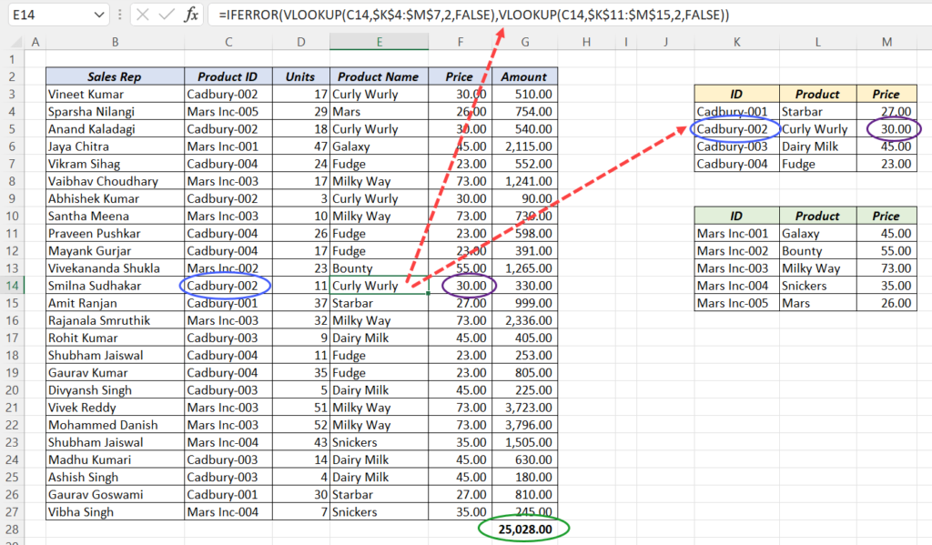
The solution to this problem is combining 2 VLOOKUP formulas using the IFERROR function.
The IFERROR function in Excel will return a ‘custom value’ when the first argument this function generates an Error and the normal result if no Error is detected.
In this case, the VLOOKUP formula to look into first table will become the first argument of the IFERROR function and the VLOOKUP formula to look into second table will become the second argument.
By doing this, whenever the first VLOOKUP returns a #N/A error, the second VLOOKUP will look into the Second Table.
=IFERROR(VLOOKUP(C3,$K$4:$M$7,3,FALSE),VLOOKUP(C3,$K$11:$M$15,3,FALSE))
Once we have the Product prices, we can calculate the Total Amount by multiplying them with the corresponding number of Units.