Dependent Drop-Down List in Excel (FILTER and INDIRECT Methods)

A dependent drop-down list changes its options based on another choice: pick Vegetable in the first list, and the second list shows only vegetables. In Excel 365, FILTER builds the second list automatically. In older versions, use named ranges with INDIRECT.

fx=FILTER(C3:C11,B3:B11=E3)

ProblemMake a drop-down list depend on another one

Functions usedData Validation, FILTER, INDIRECT

Works inAll versions (FILTER method needs 2021 or 365)

What you’re building

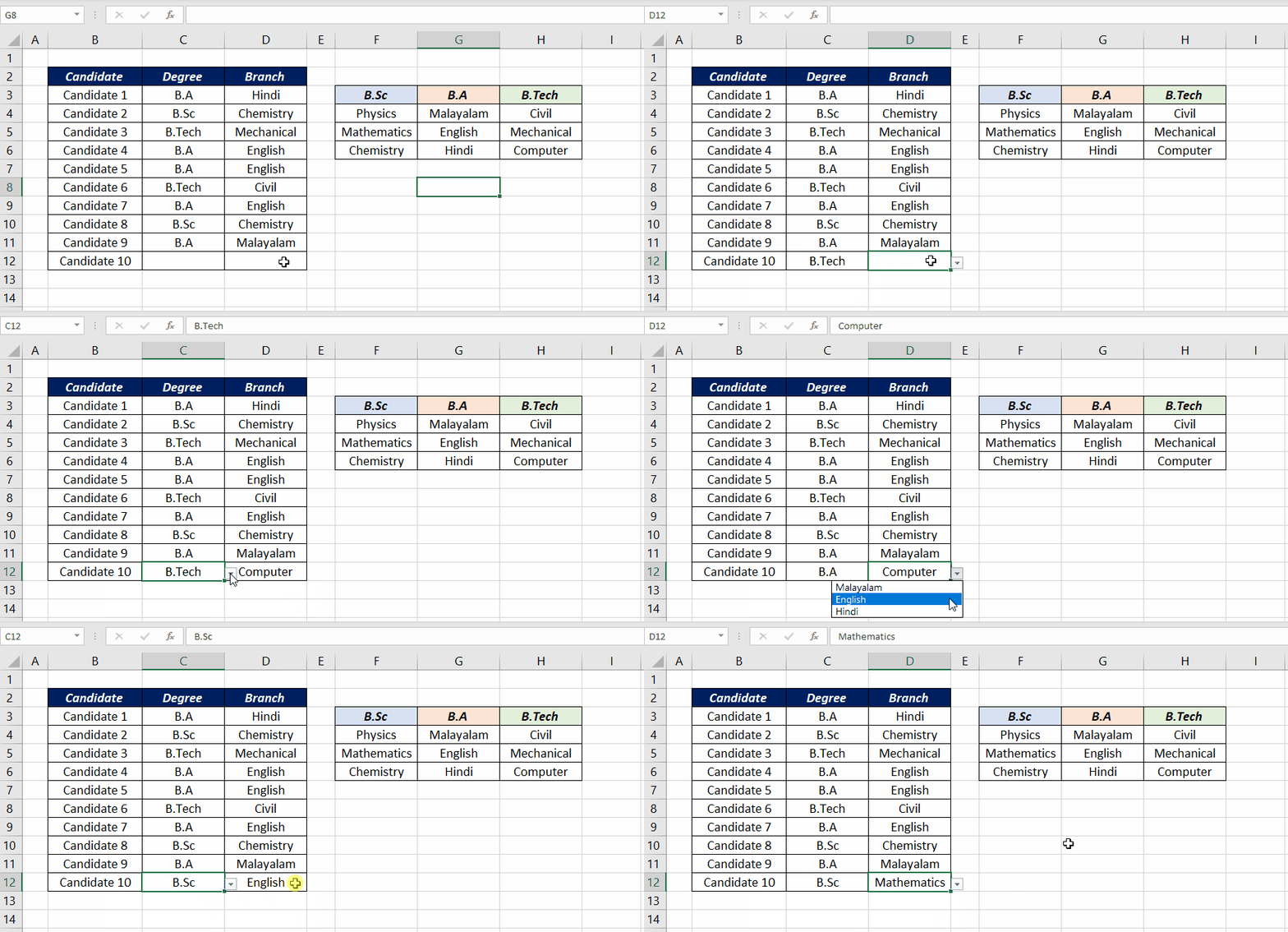
Dependent drop-down list: choosing a degree changes the list of branches

Choose B.Sc in the first list and the second shows Physics, Mathematics and Chemistry; choose B.Tech and it shows Civil, Mechanical and Computer.

Excel 365: FILTER and a spill range

Keep the data as one list of categories and items. A FILTER formula in H3 returns the items for the category chosen in E3:

=FILTER(C3:C11,B3:B11=E3)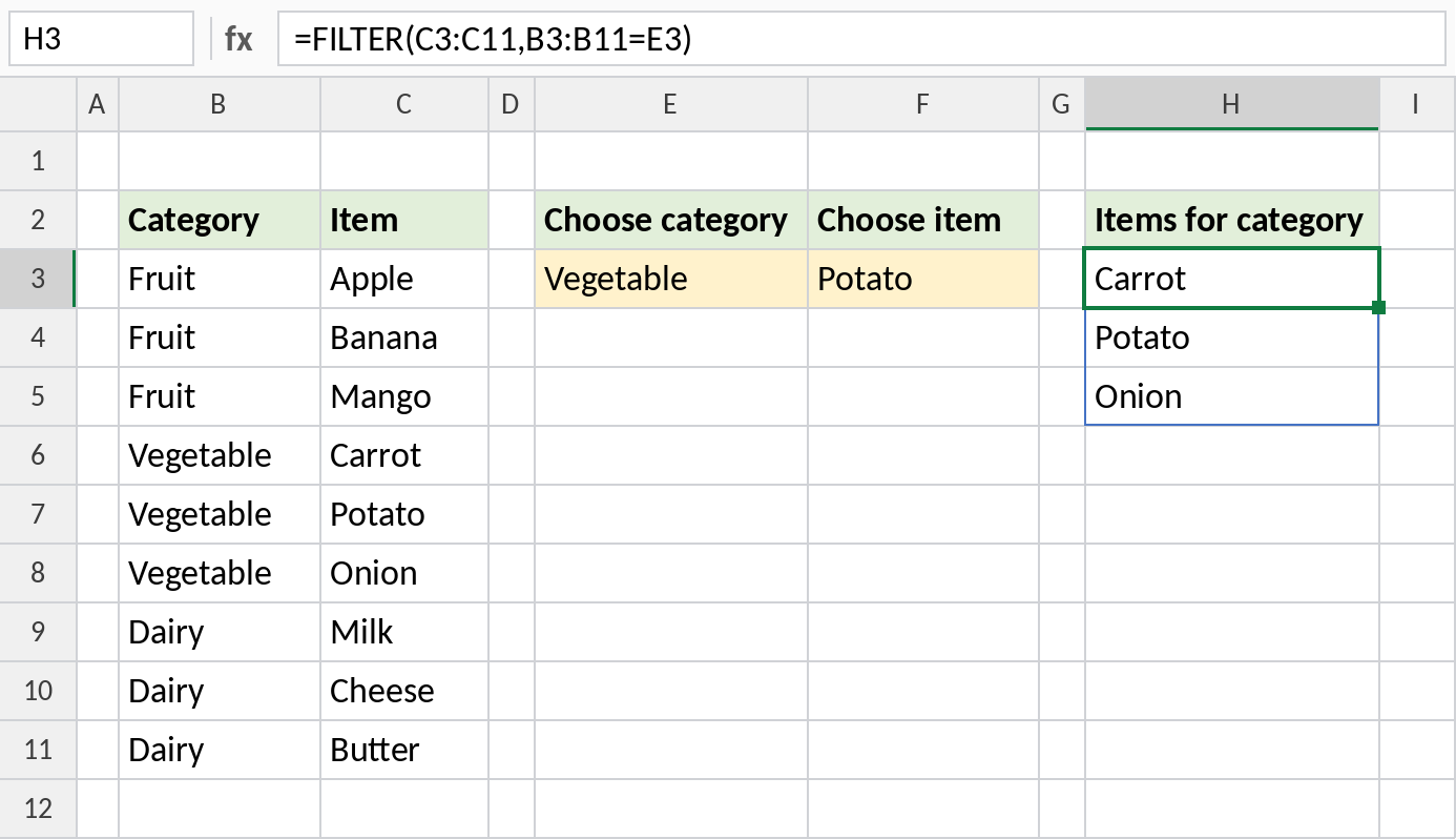

Excel FILTER returning the items for the selected category for a dependent drop-down list

With Vegetable chosen, H3 spills Carrot, Potato, Onion. Now point the second drop-down at that spill range, as shown in the steps below.

How the formula works

Make the first list: select E3 → Data → Data Validation → Allow: List → Source: Fruit,Vegetable,Dairy.
Build the item list: in H3, enter =FILTER(C3:C11,B3:B11=E3).
Make the second list: select F3 → Data Validation → List → Source: =$H$3#. The # means “the whole spill range”, so the list grows or shrinks with the category.

Any version: named ranges and INDIRECT

Put each category’s items in its own column and name each range exactly like its category: Fruit, Vegetable, Dairy. The second drop-down’s source is then:

=INDIRECT($F$3)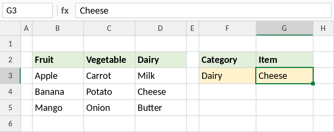

Excel dependent drop-down list using named ranges and INDIRECT

With Dairy chosen in F3, INDIRECT turns the text “Dairy” into the named range Dairy, so the list in G3 shows Milk, Cheese, Butter.

Step by step with Create from Selection

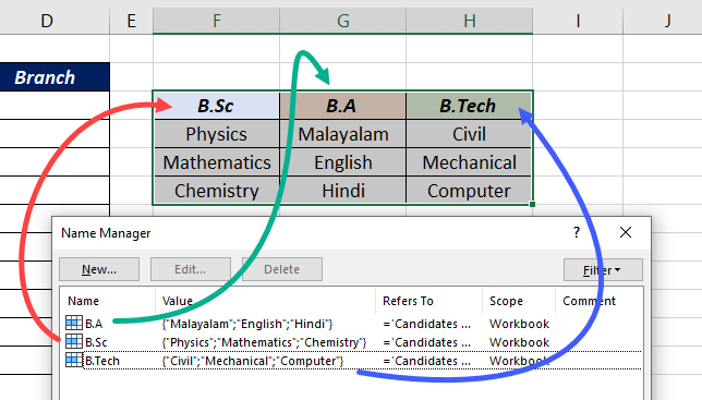
In this example the degrees are headings in F3:H3 and each degree’s branches are listed below its heading.

Select the cells for the first list → Data → Data Validation.

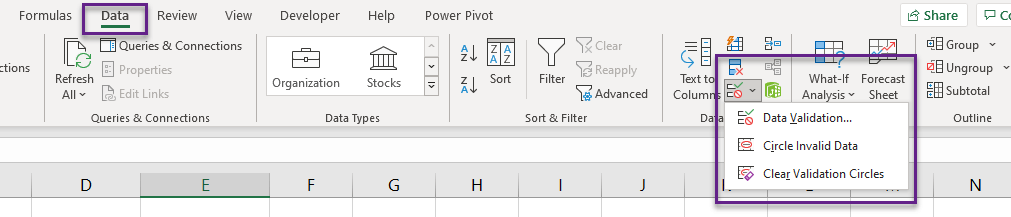
Allow: List. Source: the headings, =$F$3:$H$3. Click OK.

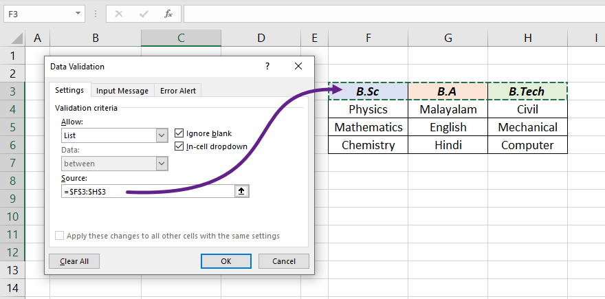
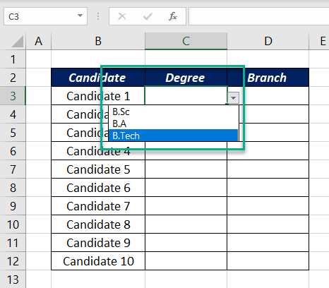
Data Validation source set to the degree headings F3:H3

First drop-down list showing B.Sc, B.A and B.Tech

Select the whole table F3:H6 → Formulas → Create from Selection → tick Top row only → OK.

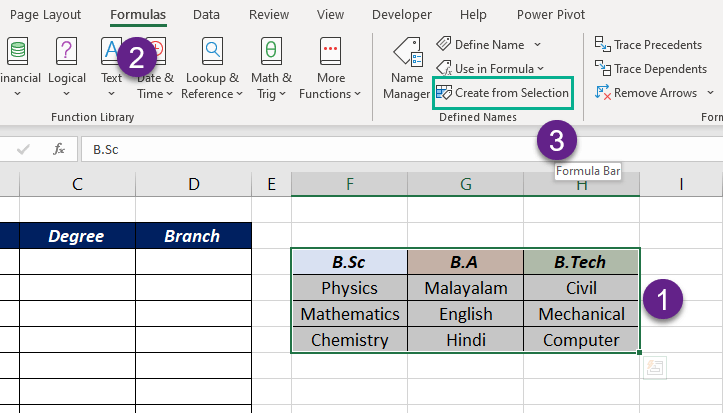
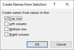
Create from Selection on the Formulas tab

Create Names from Selection dialog with Top row ticked

This creates three named ranges, B.A, B.Sc and B.Tech, each holding the branches below its heading.

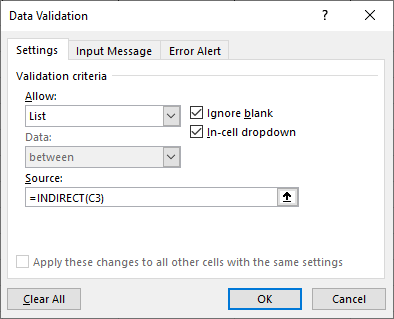
Name Manager showing the three named ranges

Select the cells for the second list → Data Validation → List → Source: =INDIRECT(C3), where C3 is the first list’s cell in that row.

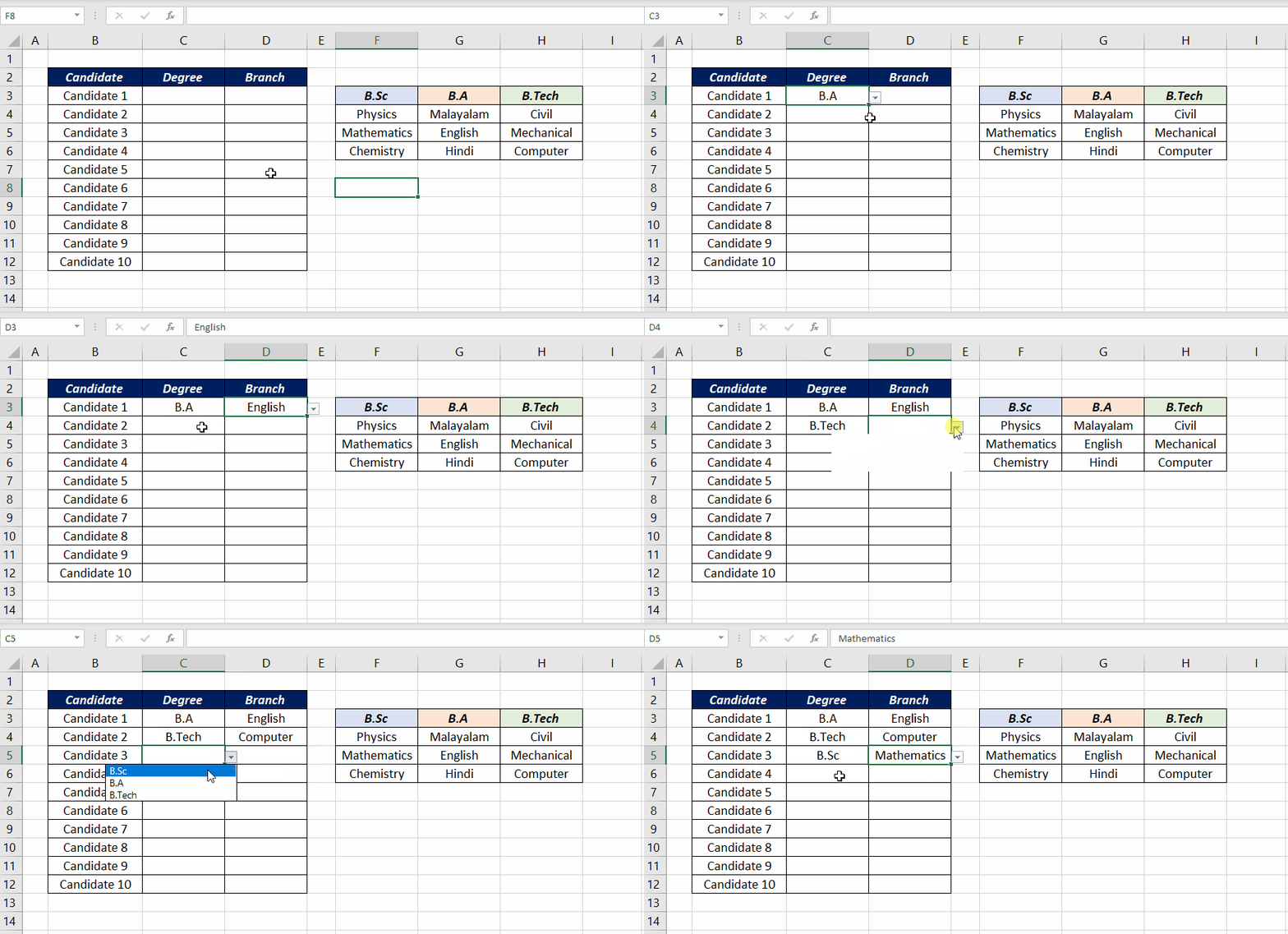
Data Validation source set to INDIRECT(C3)

The second drop-down list changing with the first

Which method to use

	FILTER method	INDIRECT method
Works in	Excel 2021, 365	All versions
Data layout	One list: category and item	One column per category
Adding items	Add a row	Extend the named range
Category names	Any text	No spaces; must match the range names

Notes

If the first choice changes, the second cell keeps its old value. Add a check such as =COUNTIF(H3#,F3)=0 with conditional formatting to flag it.
Turn the source data into an Excel Table so new items are picked up automatically.
Named ranges can’t contain spaces. For categories such as “Soft drinks”, name the range Soft_drinks and use =INDIRECT(SUBSTITUTE(F3," ","_")).

Common errors

Problem	Cause	Fix
The second list is empty	Nothing chosen in the first cell yet	Choose a category first
Source error in Data Validation	Spill reference typed without #	Use =$H$3#
INDIRECT list doesn’t work	Range name doesn’t match the category text	Check the names in Formulas → Name Manager

Practice file

Both methods with working drop-down lists.

Download .xlsx