If you are a person who use Excel a lot, you might have encountered with these Error Codes like #DIV/0!, #NAME?, #N/A, etc.
Each of these error codes tell us something. It gives us information on how to troubleshoot an incorrect formula.
Following are the most common Error codes in Excel and this blog post covers each Formula Error in detail with examples.
#DIV/0!, #NAME?, #N/A, #NUM!, #VALUE!, #REF!, #NULL!, #####, #FIELD!, #SPILL! & #CALC!
Table of Contents
#DIV/0! Error
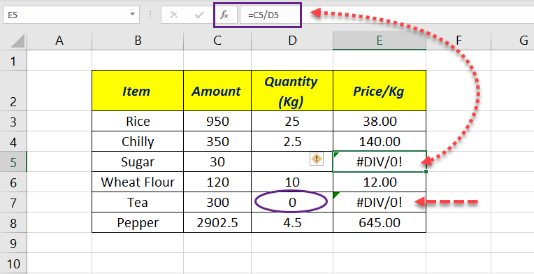
An Excel formula returns #DIV/0! when you try to divide something with zero.
In the following example, the formula =C5/D5 returns #DIV/0! error as the cell D5 is empty. The reason being Excel evaluates empty cells as Zero.
Again the same formula in the cell E7 returns #DIV/0! error as the formula is trying to divide 300 (C7) by Zero (D7).
How to fix #DIV/0 error?
Either get rid of the blank cells or use IFERROR function to trap #DIV/0 error.
#NAME! Error
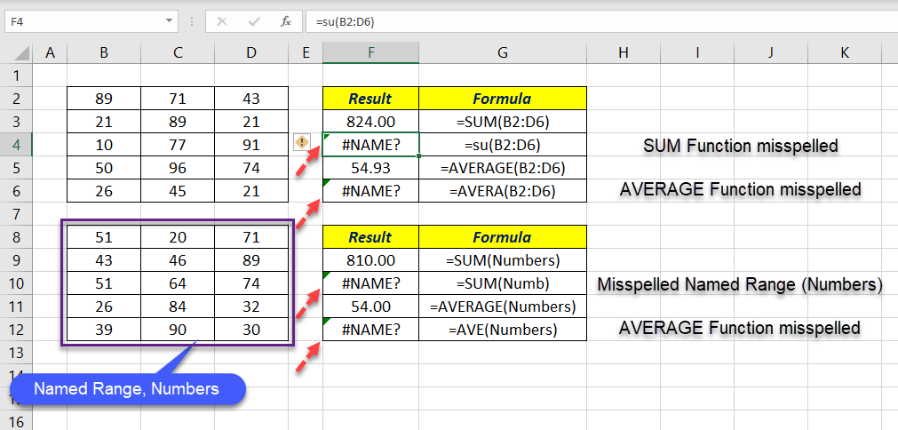
Excel returns a #NAME! error when it cannot recognize the Function or Named Range used in the formula.
In the following example, the formula returns #NAME! error, when SUM function is misspelled as SU and when AVERAGE function is misspelled as AVERA or AVE. Unrecognized Named Ranges (Numbers in this case) will result #NAME! error.
How to fix #NAME! error?
Check the spellings of the Functions and make sure the Named Ranges specified inside formulas exist.
#NA! Error
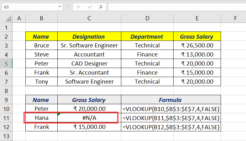
#NA! error can be read as Not Available error. Excel formulas return #NA! error when it cannot find the value specified inside the function.
#N/A! are returned by the lookup functions like VLOOKUP, HLOOKUP, MATCH, INDEX, etc.
How to fix #NA! error?
Make sure that the lookup values exist inside the lookup_table or lookup_array, otherwise use the IFERROR function to trap the #NA! error.
#NUM! Error
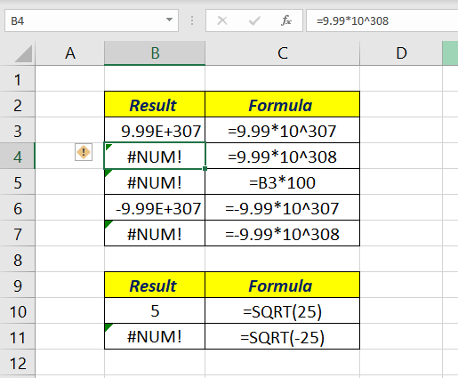
The largest number allowed in Excel is 9.99*10^307. When we try to enter a number greater than this, Excel will return a #NUM! Error. The same will be the result with the negative version of this number. Excel will return #NUM! error when we force Excel to deal with a number smaller than -99.10^307.
Another instance when an Excel formula results in #NUM! error, is operation with imaginary numbers (√-2).
For example =SQRT(-25) will result in #NUM! error
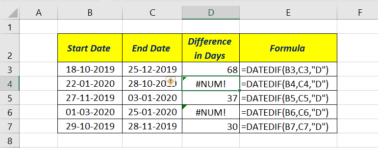
Unlike DAYS function, DATEDIF function will return #NUM! when the Start and End Dates are reversed.
How to fix #NUM! error?
Modify the inputs and make sure that the numbers used inside the formula are within the limits of Excel.
#VALUE! Error
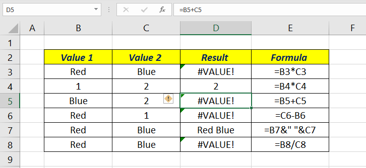
Wrong use of different Data types or Mixing of different Data types result in #VALUE! error.
For example, when you try to Multiply a Text with a Number or Add a Date to a Text, that formula will return #VALUE! error.
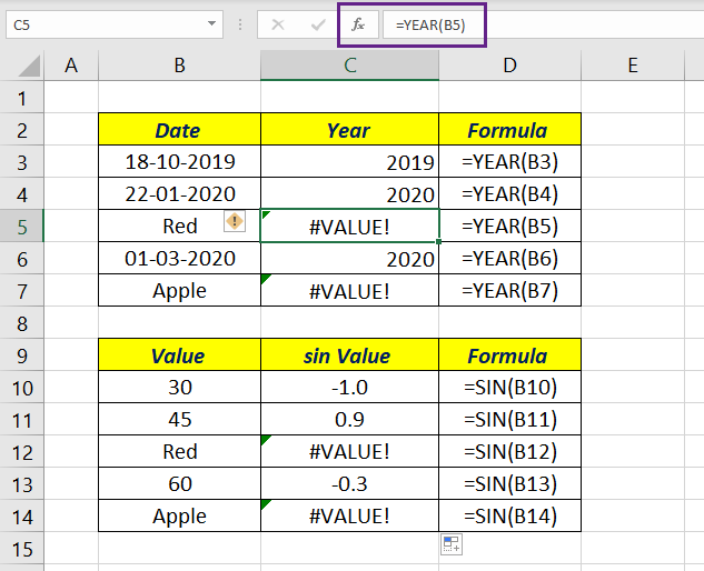
When a Text value is used inside a DATE & TIME function or a TRIGONOMETRIC function, formula will return #VALUE! error.
How to fix #VALUE! error?
Track down the problematic value and use the correct Data Type.
#REF! Error
#Ref! error appears when the cell reference or range reference becomes invalid. This happens when we delete a Row, Column or Sheet referred inside a formula.
Formulas with relative references will also return #REF! error, when copied to locations where the references update to become invalid.
In the following example, when the formula in the cell E9 is copied to G4, relative references inside the formula update accordingly and returns #REF! error.
How to fix #REF! error?
As soon as you encounter a #REF! error, press CTRL +Z or click on the Undo button to cancel that action. Otherwise if you save the workbook, the original references will be gone forever.
#NULL! Error
#NULL error appears when we use (accidentally or deliberately) the ‘Space’ character in between cell references or range references.
Space character functions as ‘Intersection Operator’ in Excel and will return the value from the cells common to the ranges specified inside the formula. In the following example, =SUM(B3 B8) returns #NULL error as the cell references B3 and B8 doesn’t intersect.
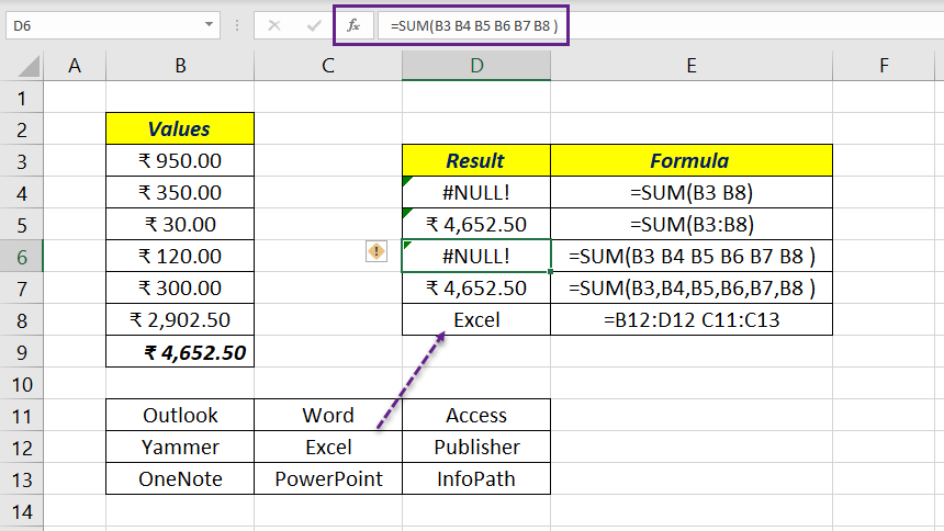
The formula =B12:D12 C11:C13 returns the value ‘Excel’ from the cell C12, as the ranges B12:D12 and C11:C13 intersect at C12
How to fix #NULL! error?
#NULL error can be avoided by replacing the Space character with Comma ‘,’ or Colon ‘:’ as required.
##### Error
Sometimes you may see that a cell or cells display a series of hash (#####) sign. Technically it is not an error and it says the cell is not wide enough display the value inside that cell or cells.
How to fix ##### error?
By increasing the width of the cell or column, we can get rid of ##### error.
#FIELD Error
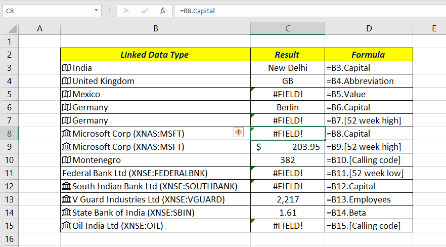
#FIELD Error is related to the Rich Data Types in Excel. At present, Stocks and Geography are the two linked data types available to the regular Excel users.
A formula will return a #FIELD! error when the referenced field doesn’t apply to the linked data type. In the following example, =B6.Capital returns Berlin whereas =B7.[52 week high] returns a #FIELD! error. Similarly, =B8.Capital returns a #FIELD! error whereas =B9.[52 week high] returns $203.95
How to fix #FIELD! error?
Make sure that the referenced field apply to the linked data type used in the formula.
#SPILL! Error
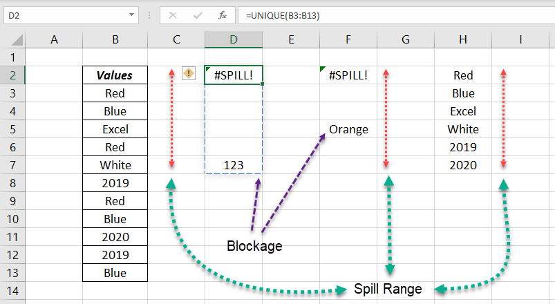
Excel formula will return a #SPILL! error when any of the cell in the spill range contains data. In other words, #SPILL! error appears when the spill range isn’t blank.
In the following example, the formula =UNIQUE(B3:B13) is used in the cells D2, F2 and H2. In the first two cases, formula returns #SPILL! error as the spill range (D2:D7 and F2:F7) contains an occupied cell each. The value ‘123’ in the cell D7 and ‘Orange’ in F5.
As the spill range from H2:H7 is empty, =UNIQUE(B3:B13) returns the unique list of values from B3;B13 into the cell H2.
How to fix #SPILL! error?
Remove the blockage in the spill range. In other words, delete the values in the spill range.
#CALC! Error
Excel returns a #CALC! error when we try to perform a calculation which isn’t supported by the calculation engine of Excel.
Excel can’t return an empty array. Whenever the calculation results in an empty array, #CALC! error will be the result.
In the following example, FILTER function is used to filter the records related to a particular product. When the name of a product (Galaxy), which is not the array of products is used inside the formula, result is an empty array and formula returns #CALC! error.
In connection with the new STOCKHISTORY function, 2 new errors #BUSY! and #BLOCKED! have been introduced into Excel.
#BUSY! says, Excel is busy collecting the data and this error disappears quickly.
#BLOCKED! error appears when the data, we are trying to retrieve is not available. For example, if you try to use a stock name which is not listed in the corresponding stock exchange, this will result in #BLOCKED! error.
You can also check this article on Formula errors in Excel
Excel Functions in Alphabetical Order (Complete list)
Complete List of Excel Functions (Category wise)
New Dynamic Array Functions in Excel