To shade every other row, use conditional formatting with =MOD(ROW(),2)=0. The banding stays correct when you insert, delete or sort rows, unlike colouring rows by hand.
Shade every other row
Select the data → Conditional Formatting → New Rule → Use a formula:
=MOD(ROW(),2)=0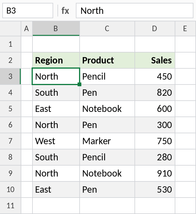
Even-numbered rows are shaded grey. Use =MOD(ROW(),2)=1 to shade the odd rows instead.
How the formula works
ROW()returns the row number of each cell: 3, 4, 5…MOD(ROW(),2)is the remainder after dividing by 2: 1 for odd rows, 0 for even rows.=0makes the rule TRUE on even rows, so only those are shaded.
Shade every third row
Change the 2 to any number for wider bands. Subtracting 2, the header row, starts the count at the first data row:
=MOD(ROW()-2,3)=0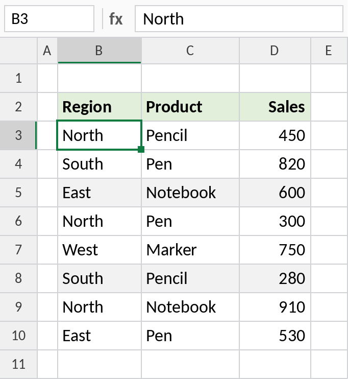
Every third data row is shaded: rows 5 and 8.
Banding options
| To | Use |
|---|---|
| Keep banding correct when filtering | =MOD(SUBTOTAL(3,$B$3:$B3),2)=0 |
| Shade every other column | =MOD(COLUMN(),2)=0 |
| Banding with one click | Convert to an Excel Table (Ctrl+T) with Banded Rows ticked |
An Excel Table gives you banding plus filters, a total row and formulas that fill down. It’s usually the best option for a list.
Step by step in the dialog
- Select the data, not the headings.
- Home → Conditional Formatting → New Rule → Use a formula to determine which cells to format, and type the formula.
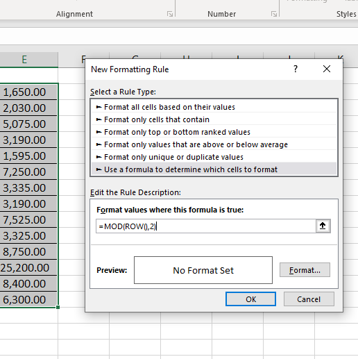
- Click Format…, choose a fill colour on the Fill tab and click OK.

- The dialog shows a preview of the format. Click OK.
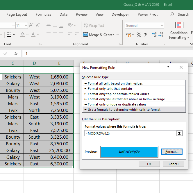
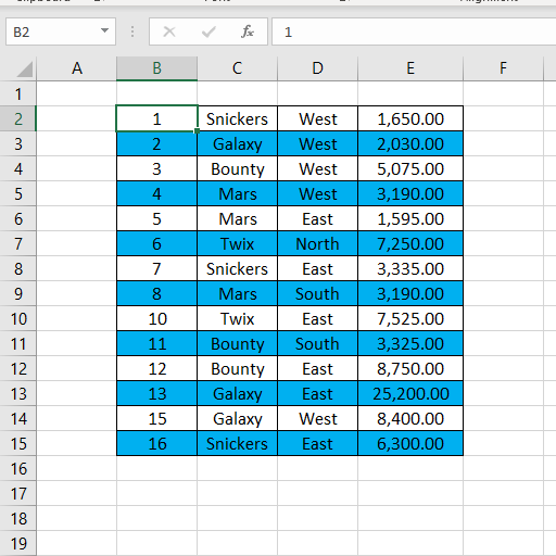
Here the rule is =MOD(ROW(),2) without =0, which shades the odd-numbered rows. Any formula that returns 1 or TRUE works as a rule.
Method 2: an Excel Table
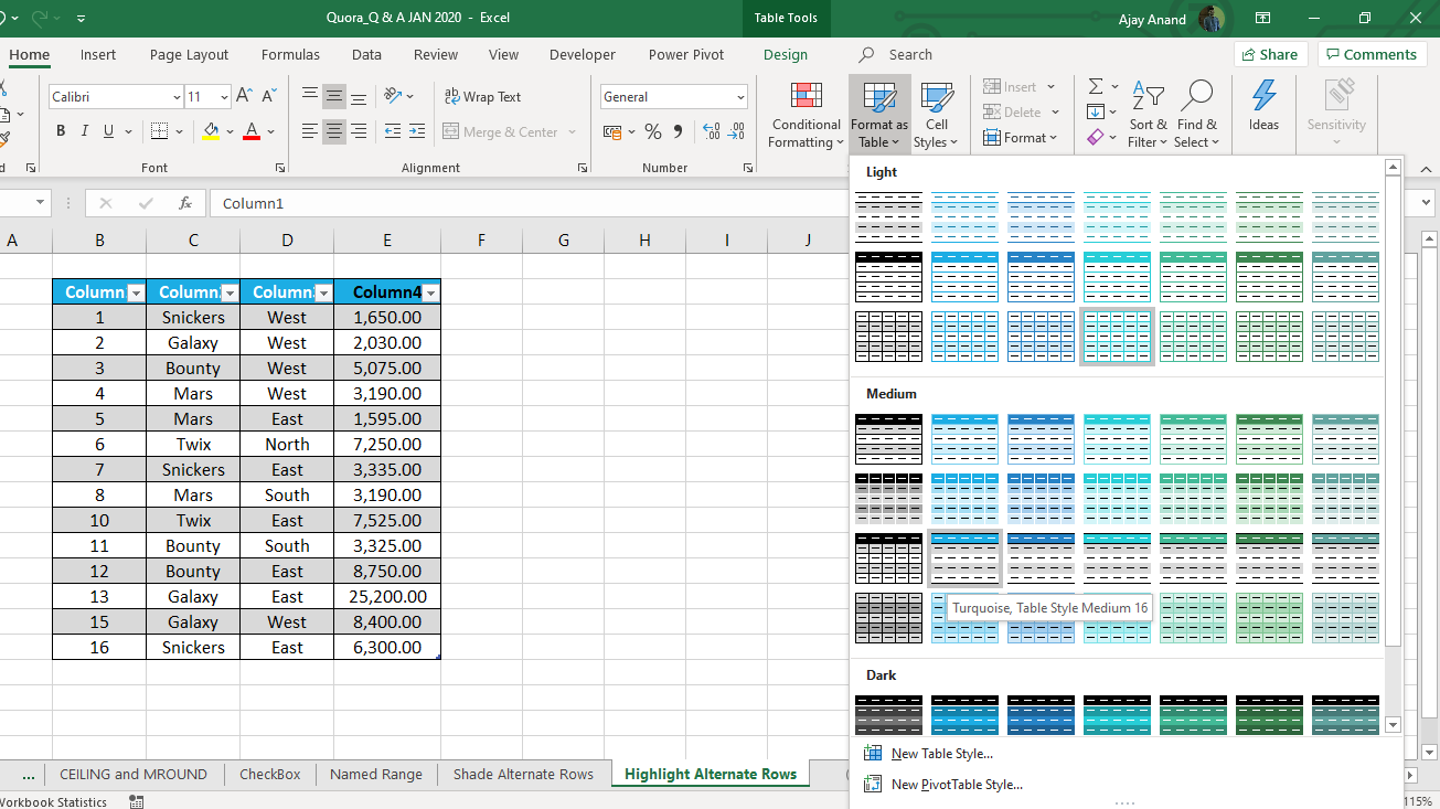
If the list will grow, convert it to an Excel Table. New rows get the banding automatically.
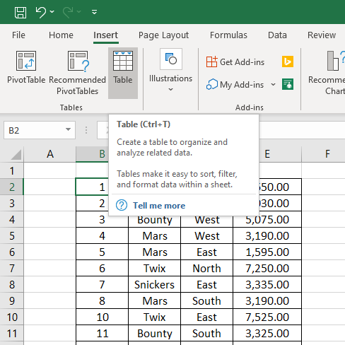
- Click any cell in the data → Insert → Table (or Ctrl + T).
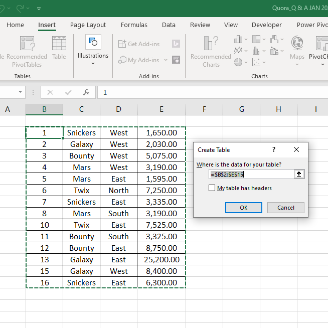
- Check the range and My table has headers, then click OK.
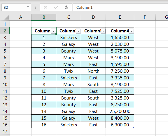
- To change the colours, pick a style from Home → Format as Table or Table Design → Table Styles.
Notes
- With a normal MOD rule, filtered rows can leave two shaded rows next to each other. The SUBTOTAL version counts only visible rows.
- Choose a light fill so text stays easy to read, and print-friendly.
- Conditional formatting colours override fills you’ve added by hand.
Common errors
| Problem | Cause | Fix |
|---|---|---|
| Banding breaks after filtering | MOD(ROW()) counts hidden rows | Use the SUBTOTAL version |
| The header is shaded | Rule applied to the header row | Start the selection at the first data row |
Practice file
Both rules are set up in the practice file.