To list the top 3, top 5 or top N records with a formula, sort the data by value and keep the first N rows. In Excel 365 that’s one formula with SORT and TAKE. In older versions, use LARGE with INDEX and MATCH.
Excel 365: SORT and TAKE
SORT puts the rows in descending order by the third column, Sales. TAKE keeps the first 3:
=TAKE(SORT(B3:D10,3,-1),3)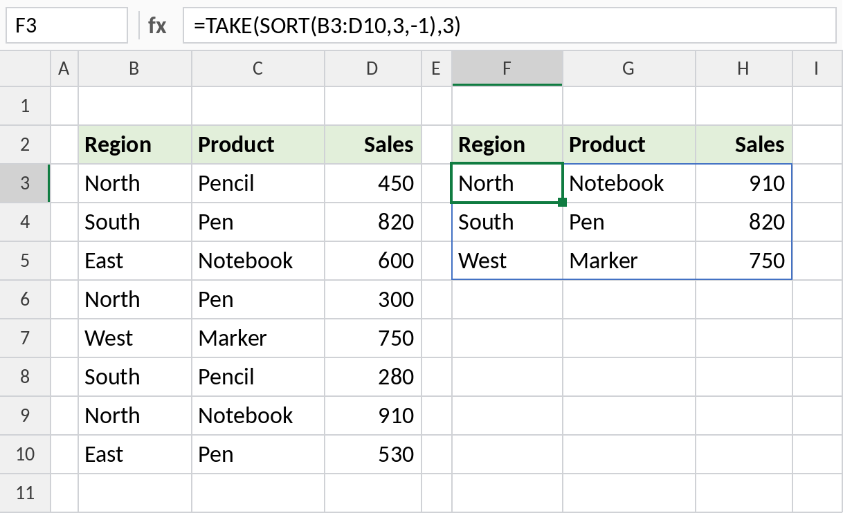
The top three rows spill out, led by North Notebook with 910. Change 3 to 5 for a top 5.
How the formula works
SORT(B3:D10,3,-1)sorts the table by column 3, Sales, in descending order (-1).TAKE(…,3)keeps the first 3 rows of the sorted result.- Because it spills, the list updates whenever the data changes.
Any version: LARGE with INDEX and MATCH
LARGE returns the 1st, 2nd and 3rd largest sales, using the rank in column F. INDEX and MATCH then find the product for each value:
=LARGE($D$3:$D$10,F3)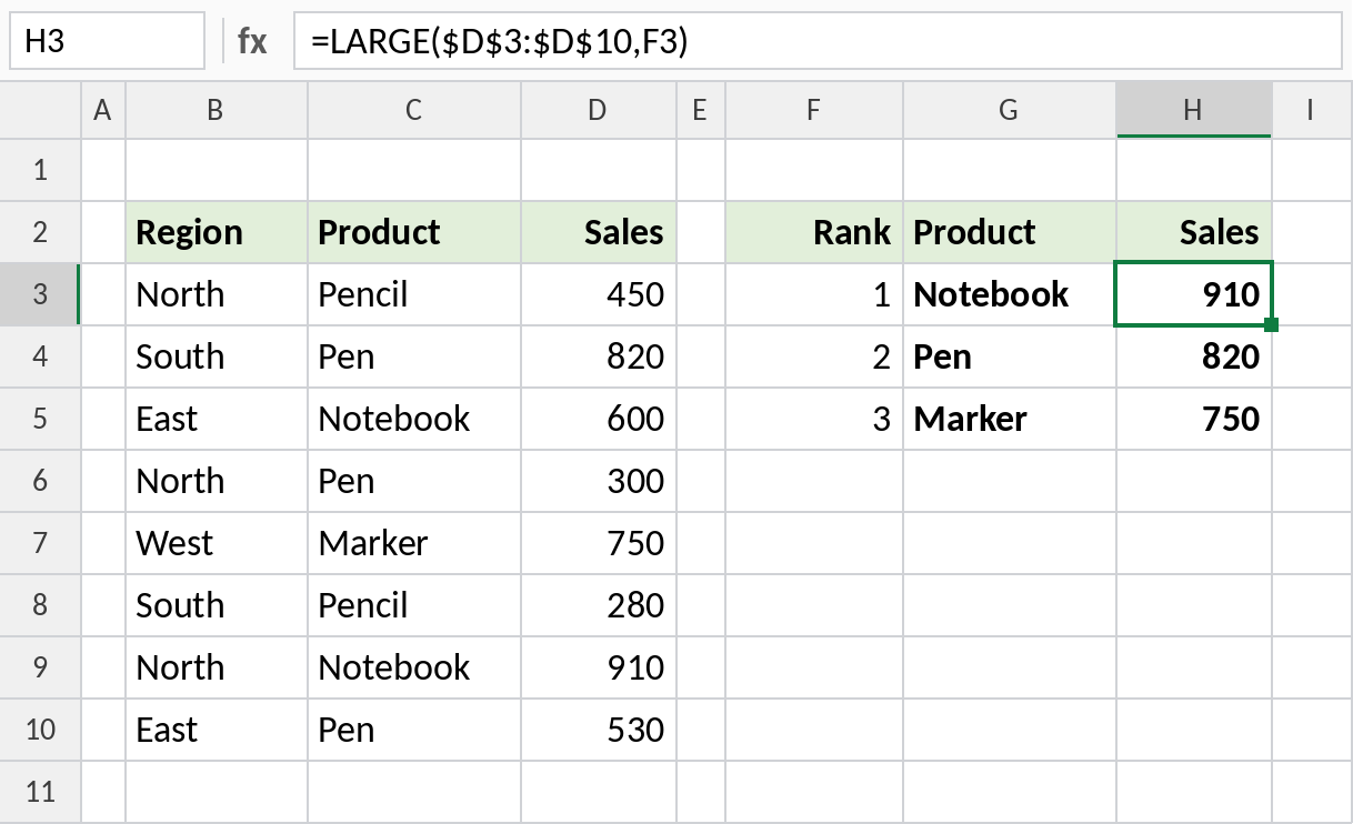
H3 returns the largest sale, 910, and G3 finds its product with =INDEX($C$3:$C$10,MATCH(H3,$D$3:$D$10,0)).
Keep the original order
To list the top 3 without re-sorting them, keep every row whose sales are at least the 3rd largest value:
=FILTER(B3:D10,D3:D10>=LARGE(D3:D10,3))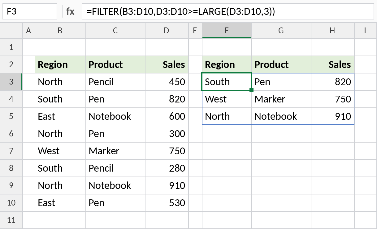
The same three rows appear, in the order they are in the table.
Variations
| To get | Formula |
|---|---|
| Bottom 3 | =TAKE(SORT(B3:D10,3,1),3) |
| Top 3 for one region | =TAKE(SORT(FILTER(B3:D10,B3:B10="North"),3,-1),3) |
| Top N from a cell | =TAKE(SORT(B3:D10,3,-1),G1) |
| Just the top 3 values | =LARGE(D3:D10,{1;2;3}) |
To add up the top values instead of listing them, see sum the top N values.
Notes
- With the INDEX/MATCH method, duplicate values return the same product twice. The SORT/TAKE method doesn’t have that problem.
- The FILTER method returns more than N rows if there’s a tie for Nth place.
- TAKE needs Excel 365. In Excel 2021, use
=INDEX(SORT(B3:D10,3,-1),SEQUENCE(3),{1,2,3}).
Common errors
| Problem | Cause | Fix |
|---|---|---|
#NAME? |
TAKE or SORT not available | Use the LARGE/INDEX method |
| Same product listed twice | Tied values with INDEX/MATCH | Use SORT and TAKE |
#SPILL! |
Cells in the way | Clear the spill range |
Practice file
All three methods in one workbook.