Excel HSTACK Function: Combine Columns Side by Side

The Excel HSTACK function places ranges side by side into one wider array. Use it to rearrange columns, add calculated columns or line up lists.

fx=HSTACK(array1, [array2], ...)

`array1`	The first range or array.
`array2, ...` optional	More ranges to add on the right, up to 254.

Table of Contents

Basic example

To show Product before Region, list the columns in the order you want:

=HSTACK(C3:C10,B3:B10)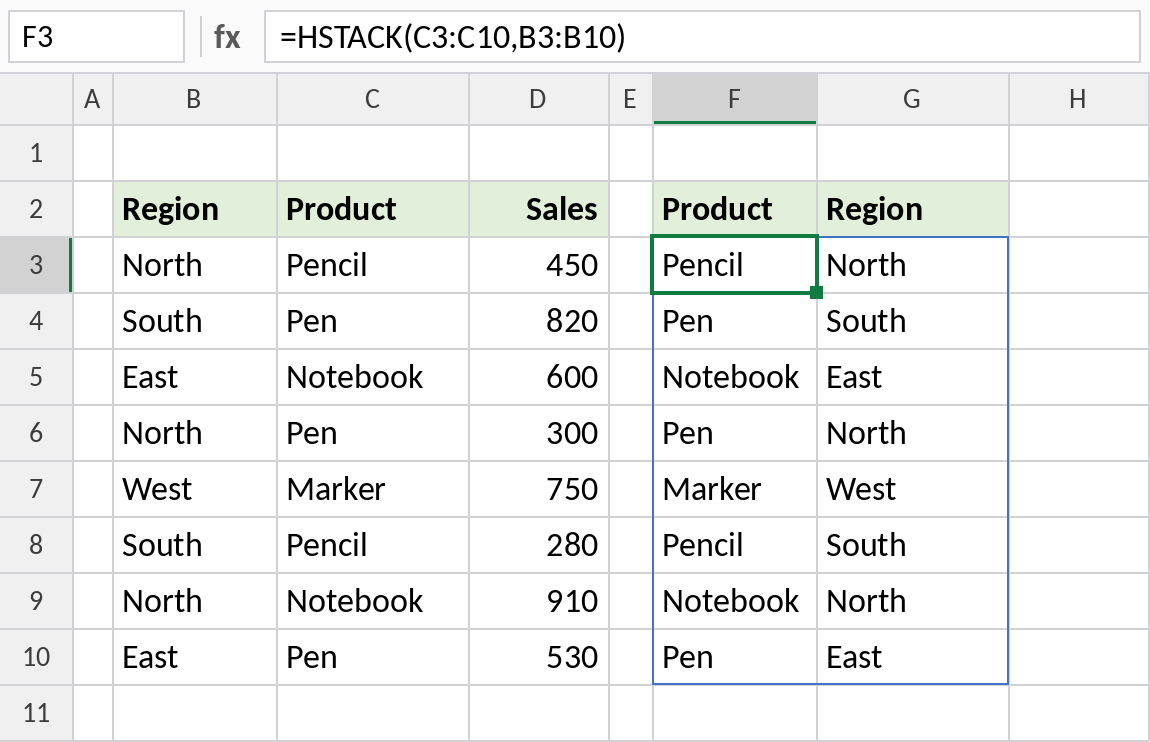

The two columns spill side by side with Product first. The original data doesn’t move.

Any argument can be a calculation. This adds a 5% commission column next to region and sales:

=HSTACK(B3:B10,D3:D10,D3:D10*5%)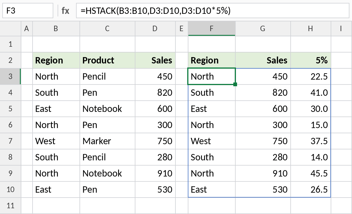

Each row shows the region, the sale and 5% of it: 450 gives 22.5. One formula builds the whole report.

Batch A has 4 names and Batch B has 3. HSTACK fills the missing cell with #N/A, so wrap it in IFNA:

=IFNA(HSTACK(SORT(B3:B6),SORT(D3:D5)),"")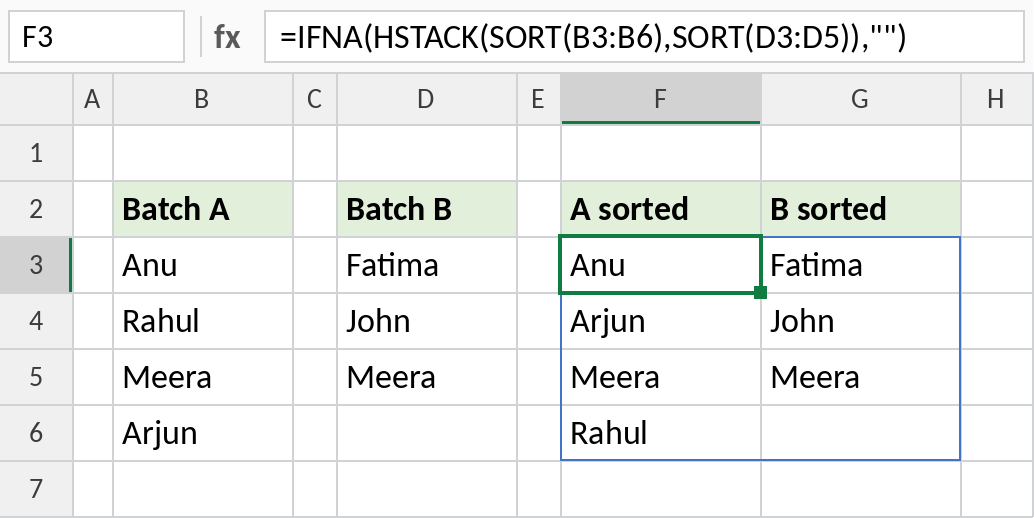

Both lists are sorted and placed next to each other. The empty spot in the last row shows as blank instead of #N/A.

	HSTACK	VSTACK
Combines	Side by side	On top of each other
Different sizes	Shorter ranges padded with #N/A below	Narrower ranges padded with #N/A on the right
Typical use	Build a report from chosen columns	Combine lists or sheets

See VSTACK for stacking lists and combining sheets.

Ranges are placed left to right in the order you list them.
If ranges have different heights, the shorter ones are padded with #N/A. Wrap in IFNA to hide it.
Combine HSTACK with CHOOSECOLS, FILTER and SORT to build a report in one formula.
The result updates automatically when the source data changes.

Problem	Cause	Fix
`#N/A` in the result	Ranges have different heights	Use `=IFNA(HSTACK(...),"")`
`#SPILL!`	Cells to the right aren’t empty	Clear them
`#NAME?`	Excel 2021 or earlier	Copy and paste the columns, or use CHOOSE with an array

Practice file

All three examples with working formulas (Excel 2024 or 365).