The Excel SUM function adds numbers. Use it to total a column, a row, several ranges at once, or a mix of cells and values.
number1 |
The first number, cell or range to add, such as C3:C8. |
|---|---|
number2, ... optional |
More numbers, cells or ranges. You can give up to 255 in total. |
Table of Contents
Basic example
To total the January sales, give SUM the range that holds them:
=SUM(C3:C8)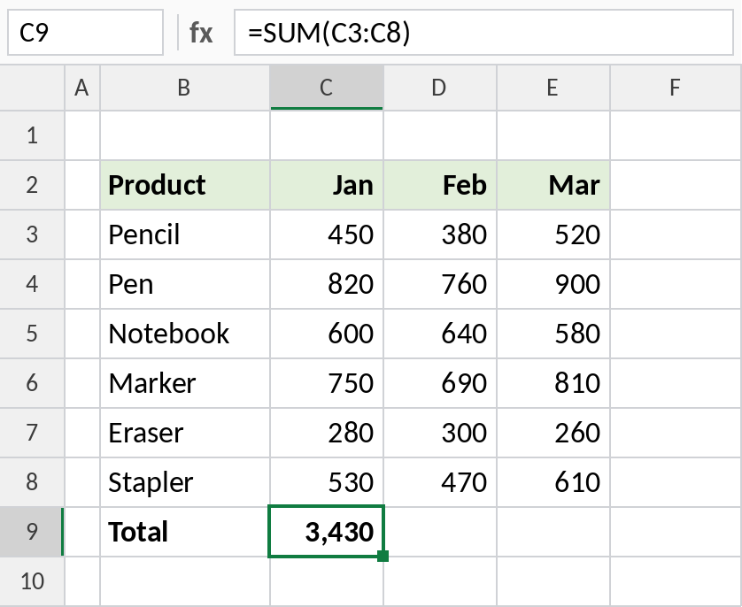
Excel adds every number from C3 to C8: 3,430. If you change any value in the range, the total updates straight away.
Sum a row
SUM works across rows the same way. To get each product’s total for the quarter, add its Jan, Feb and Mar values:
=SUM(C3:E3)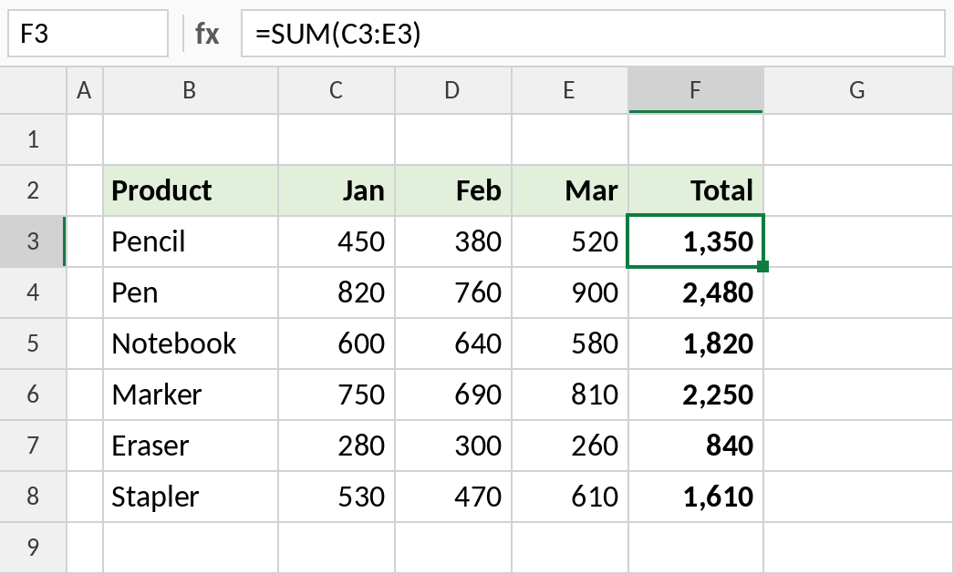
Enter the formula in F3, then drag the fill handle down to F8. The references move with each row, so F4 becomes =SUM(C4:E4), and so on.
Sum ranges that aren’t next to each other
Separate each range with a comma. This adds January and March but skips February:
=SUM(C3:C8,E3:E8) 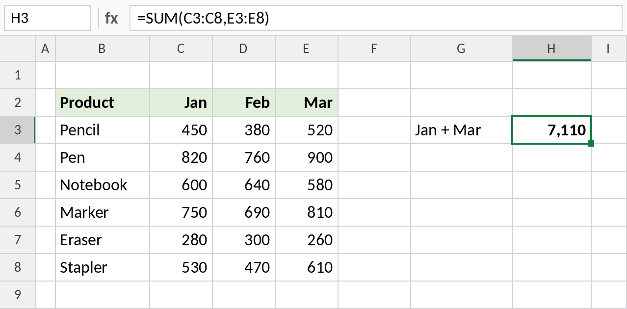
3,430 for January plus 3,680 for March gives 7,110. While typing the formula, you can hold Ctrl and select each range with the mouse instead of typing the references.
AutoSum: the fastest way
Select the empty cells just below your data, here C9:E9, and press Alt + =. Excel writes a SUM formula in each cell for you:
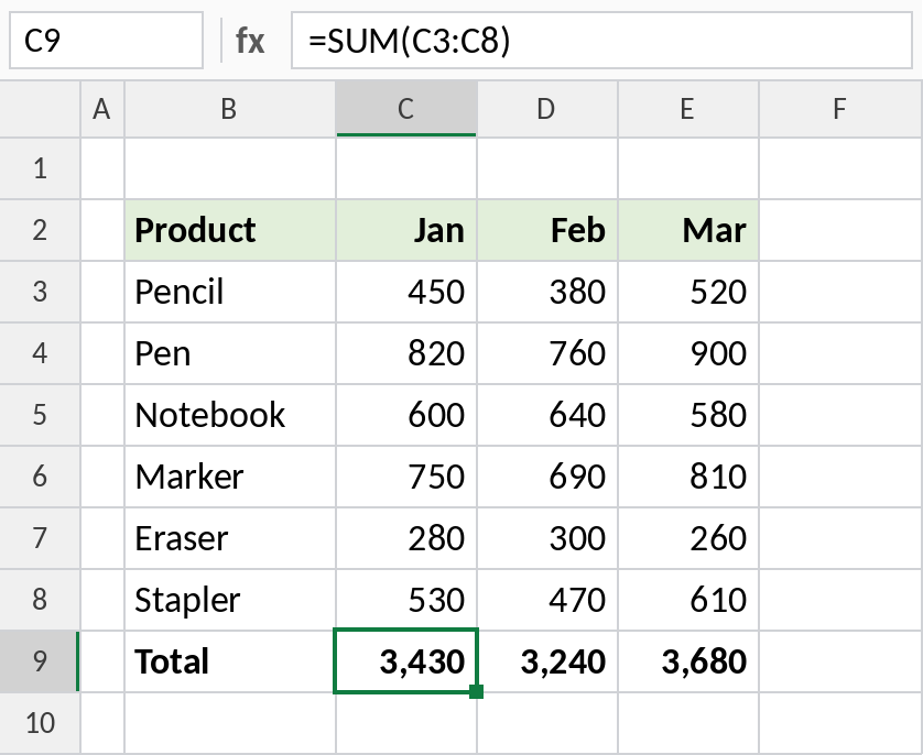
All three month totals appear in one step: 3,430, 3,240 and 3,680. AutoSum guesses the range from the data above or to the left, so check it picked the right cells. The same button is on the Home tab, at the far right.
Ways to write SUM
| Formula | What it adds |
|---|---|
=SUM(C3:C8) |
One range |
=SUM(C3:E8) |
A whole block, here all three months: 10,350 |
=SUM(C3:C8,E3:E8) |
Two separate ranges |
=SUM(C3,C5,C7) |
Individual cells |
=SUM(C3:C8,500) |
A range plus a fixed number |
=SUM(C:C) |
An entire column (keep the formula outside that column) |
=SUM(Sales[Jan]) |
A column in an Excel Table named Sales |
=SUM(Jan:Mar!C3) |
The same cell across sheets Jan to Mar (a 3D reference) |
Notes
- SUM ignores text, empty cells and TRUE/FALSE values inside ranges.
- Numbers stored as text inside a range are ignored too. They usually sit on the left of the cell with a small green triangle. Convert them to real numbers to include them.
- If any cell in the range has an error such as
#N/A, SUM returns that error. Use=AGGREGATE(9,6,C3:C8)to add the numbers and skip errors. - SUM includes hidden and filtered-out rows. To total only visible rows, use SUBTOTAL.
- To check a total quickly without a formula, select the cells and look at the Status Bar at the bottom of the window.
Common errors
| Problem | Cause | Fix |
|---|---|---|
| Total is too low or 0 | Some numbers are stored as text | Select them, click the warning icon and choose Convert to Number |
#N/A, #VALUE! |
An error cell inside the range | Fix the source cell, or use AGGREGATE(9,6,range) |
| Circular reference warning | The formula’s cell is inside its own range, such as =SUM(C3:C9) typed in C9 |
End the range one row above the formula |
| Total doesn’t update | Calculation is set to Manual | Formulas tab → Calculation Options → Automatic |
##### |
The column is too narrow for the result | Widen the column |
Practice file
All four examples, with a blank total row to try AutoSum yourself.