The Excel CHOOSECOLS function returns only the columns you pick from a range, in any order. Negative numbers count from the right.
array |
The range to pick columns from. |
|---|---|
col_num1 |
The first column to return. 1 is the first column, -1 is the last. |
col_num2, ... optional |
More columns, in the order you want them. |
Table of Contents
Basic example
To keep only Region and Sales, pick columns 1 and 3:
=CHOOSECOLS(B3:D10,1,3)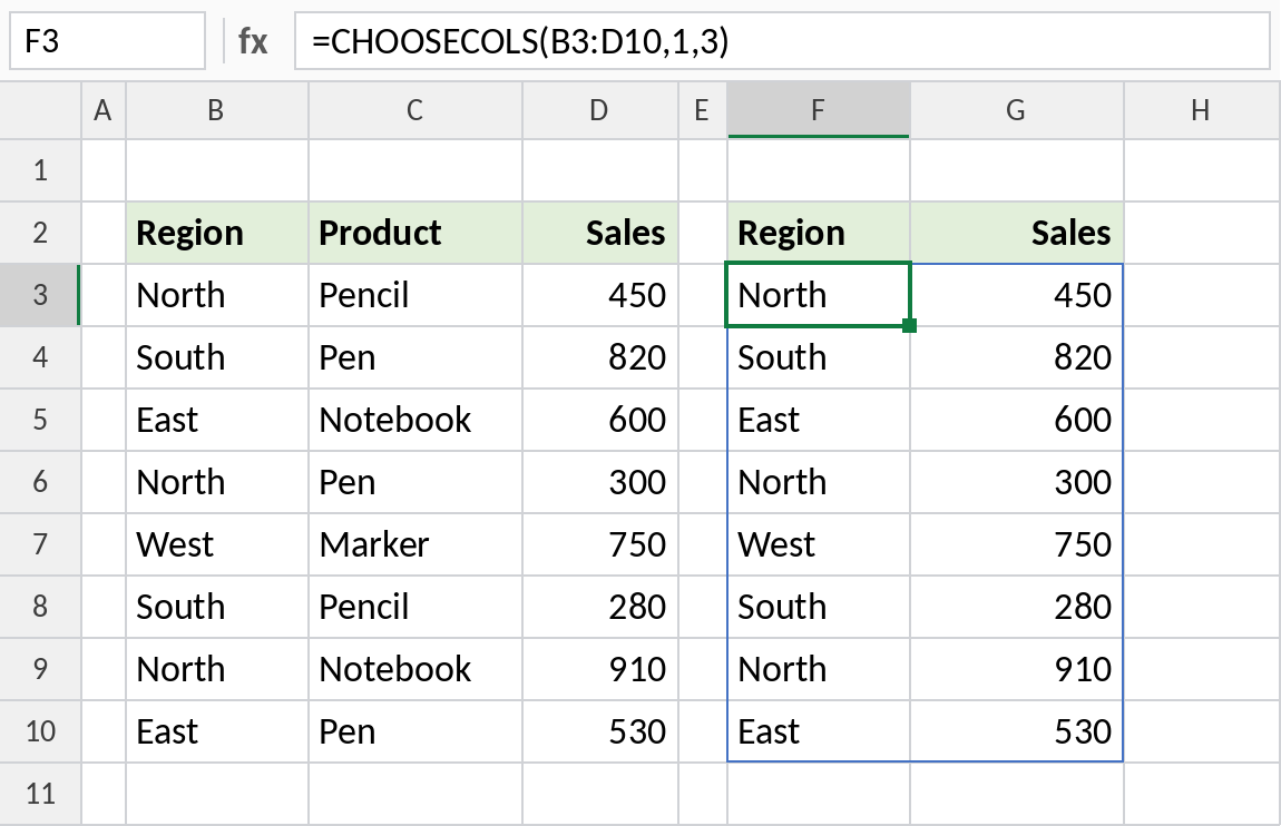
The Product column is left out. North and 450 head the result, and the whole thing updates with the source.
Pick columns from FILTER results
FILTER returns all columns. Wrap it in CHOOSECOLS to drop the Region column, which is the same for every row anyway:
=CHOOSECOLS(FILTER(B3:D10,B3:B10="North"),2,3)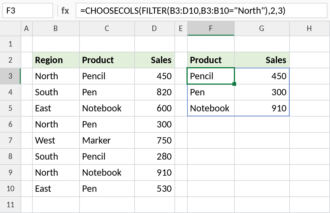
Only Product and Sales for the 3 North rows are returned.
Pick columns by header name
Column numbers break if someone inserts a column. Let XMATCH find the numbers from the header names instead:
=CHOOSECOLS(B3:D10,XMATCH({"Sales","Region"},B2:D2))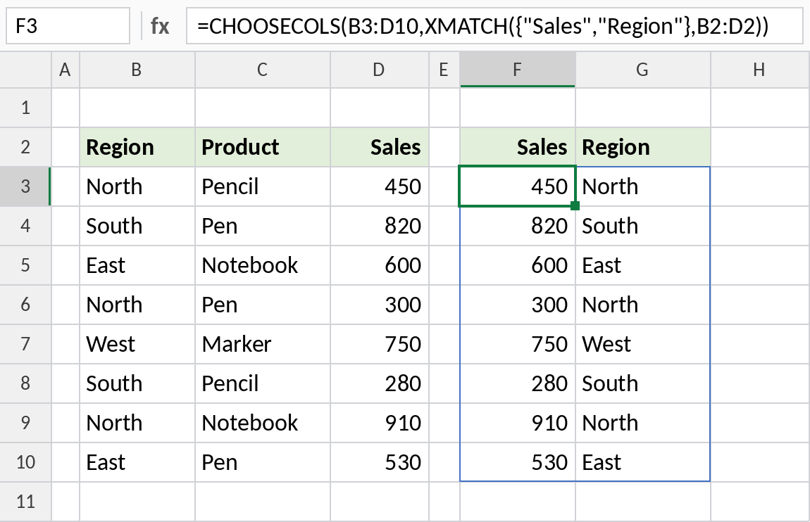
XMATCH returns 3 and 1, so the result shows Sales first, then Region. It keeps working if the source columns are rearranged.
CHOOSECOLS and its relatives
| Function | Returns |
|---|---|
| CHOOSECOLS | Chosen columns |
| CHOOSEROWS | Chosen rows, such as CHOOSEROWS(B3:D10,1,-1) for the first and last |
| TAKE / DROP | The first or last N rows or columns, or all except them |
| HSTACK | Columns from different ranges, side by side |
Notes
- Negative column numbers count from the right: -1 is the last column.
- You can repeat a column number to return it twice.
- A column number larger than the range returns
#VALUE!. - CHOOSECOLS is ideal for trimming the output of FILTER, SORT or XLOOKUP.
Common errors
| Problem | Cause | Fix |
|---|---|---|
#VALUE! |
A column number is 0 or larger than the range | Use numbers inside the range |
#SPILL! |
Cells in the spill range aren’t empty | Clear them |
#NAME? |
Excel 2021 or earlier | Copy the columns you need, or use INDEX |
Practice file
All three examples with working formulas (Excel 2024 or 365).