The Excel XLOOKUP function finds a value in one range and returns the matching value from another. It looks in any direction and has a built-in message for when nothing is found.
lookup_value |
The value to find, such as an ID. |
|---|---|
lookup_array |
The range to search. |
return_array |
The range to return a result from. |
if_not_found optional |
What to return if there’s no match. Without it, XLOOKUP returns #N/A. |
match_mode optional |
0 exact (default), -1 exact or next smaller, 1 exact or next larger, 2 wildcards. |
search_mode optional |
1 first to last (default), -1 last to first. |
Table of Contents
Basic example
To find the product name for an ID, search the ID column and return the Product column:
=XLOOKUP(H3,B3:B8,C3:C8) 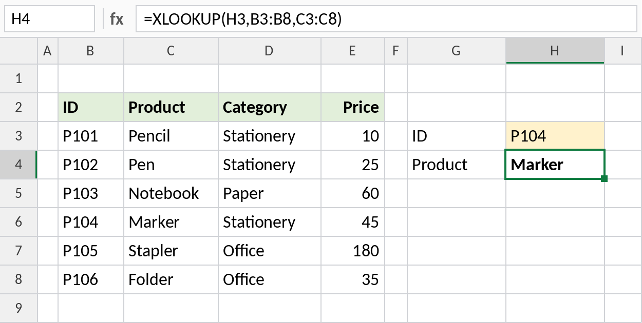
XLOOKUP finds P104 in row 6 and returns the product from the same row: Marker. Exact match is the default, so there’s no TRUE/FALSE to remember.
Look up to the left
The return range can sit on either side of the lookup range. Here, the product name finds its ID in the column to the left:
=XLOOKUP(H3,C3:C8,B3:B8) 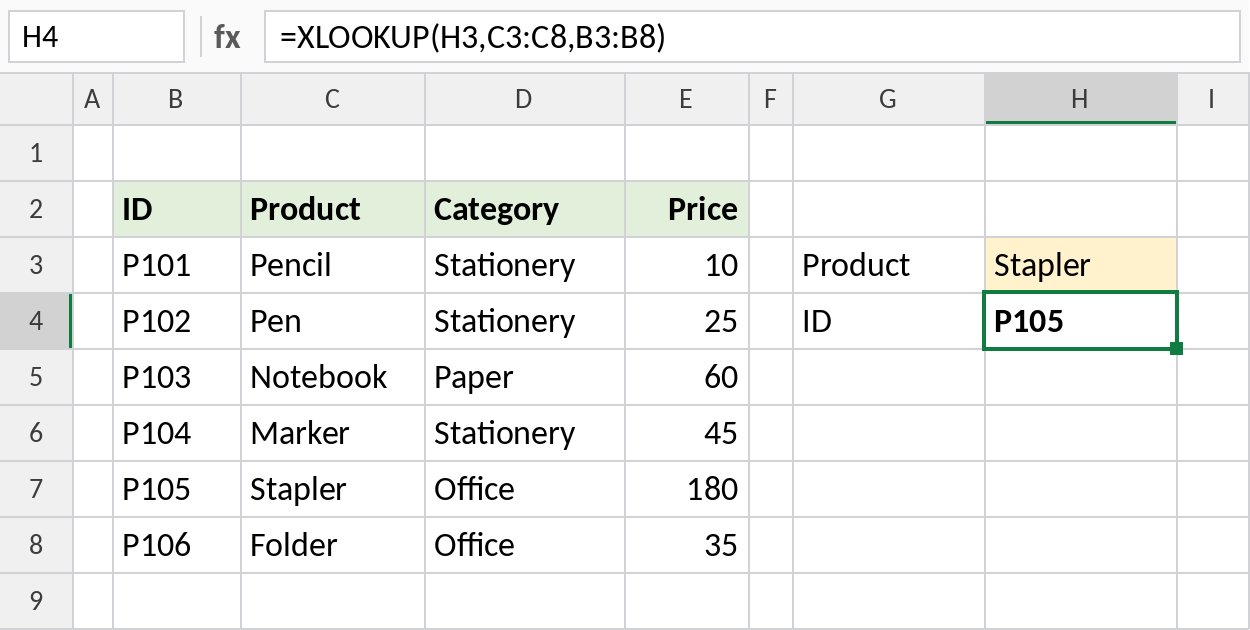
Stapler is found in the Product column, and XLOOKUP returns P105 from the ID column. VLOOKUP can’t do this, because it only returns columns to the right.
Show a message if nothing is found
Use the fourth argument to replace #N/A with your own text:
=XLOOKUP(H3,B3:B8,E3:E8,"Not found") 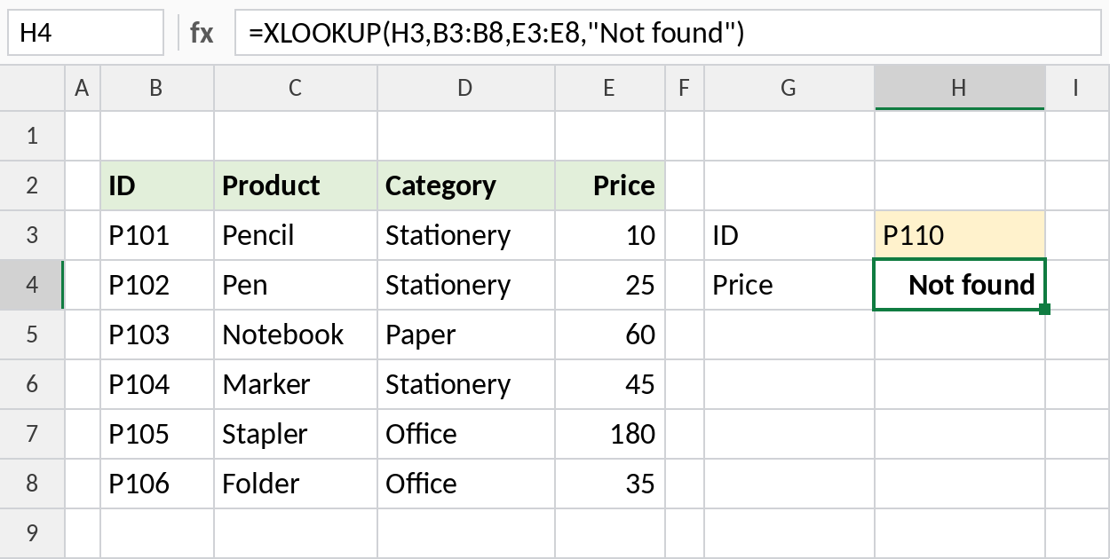
P110 isn’t in the list, so XLOOKUP returns Not found. No IFERROR wrapper is needed.
Return a whole row
Give XLOOKUP several columns as the return range, and it returns all of them at once:
=XLOOKUP(H3,B3:B8,C3:E8) 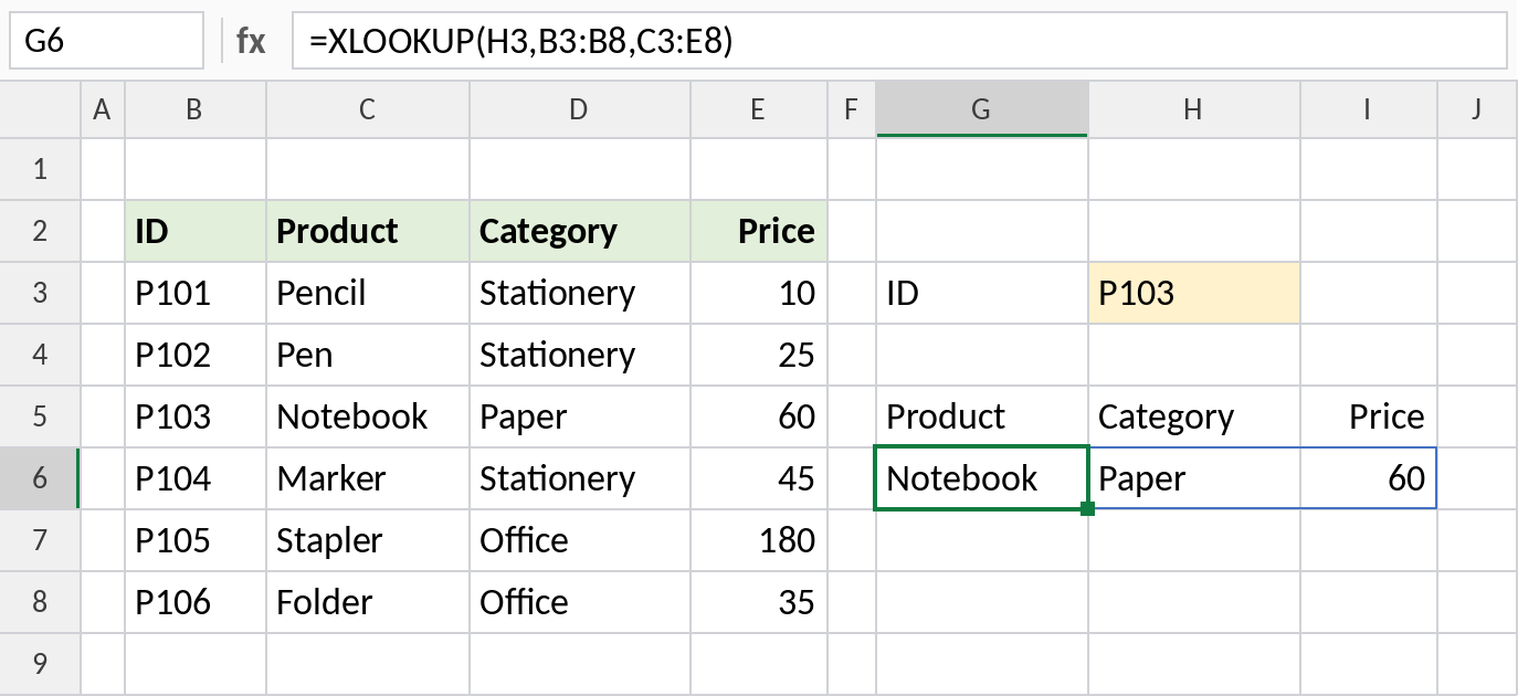
The formula is only in G6, but the results spill into H6 and I6: Notebook, Paper and 60. The blue border shows the spill range. Keep the cells to the right empty, or you’ll see #SPILL!.
XLOOKUP vs VLOOKUP
| VLOOKUP | XLOOKUP | |
|---|---|---|
| Default match | Approximate (unless FALSE) | Exact |
| Look left | No | Yes |
| Column number needed | Yes, breaks if columns move | No |
| Not-found message | Needs IFERROR | Built in |
| Return several columns | One at a time | Yes, spills |
| Available in | All versions | 2021 and later, 365 |
Notes
- Exact match is the default. Use
match_mode-1 or 1 for approximate matches, such as tax slabs. lookup_arrayandreturn_arraymust have the same number of rows.- Set
search_modeto -1 to find the last match instead of the first. - If you share files with people on Excel 2019 or earlier, use INDEX and MATCH instead.
Common errors
| Problem | Cause | Fix |
|---|---|---|
#N/A |
The value isn’t in lookup_array, often because of extra spaces or numbers stored as text |
Add if_not_found, and clean the data with TRIM |
#VALUE! |
lookup_array and return_array are different sizes |
Make both ranges cover the same rows |
#SPILL! |
Cells in the spill range aren’t empty | Clear the cells the result needs |
#NAME? |
Opened in Excel 2019 or earlier | Use INDEX and MATCH |
Practice file
All four examples with working formulas.