Excel FILTER Function: Multiple Criteria, AND, OR and If Empty

The Excel FILTER function returns every row that meets your conditions. The results spill into the cells below and update automatically when the data changes.

fx=FILTER(array, include, [if_empty])

Purpose: Return the rows that meet conditions
Returns: An array of matching rows that spills
Available in: Excel 2021, 2024, 365, Excel for the web, Google Sheets

`array`	The range to return rows from.
`include`	A test the same height as `array`, such as `B3:B10="North"`. Rows where it’s TRUE are kept.
`if_empty` optional	What to show if no rows match. Without it, FILTER returns `#CALC!`.

Table of Contents

Basic example

To list all North orders, give FILTER the data and a test on the Region column:

=FILTER(B3:D10,B3:B10="North")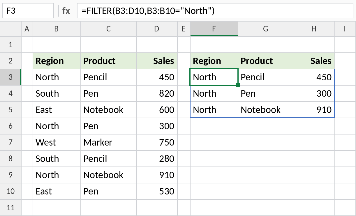

Excel FILTER returning all North rows, spilling into three rows

The formula sits only in F3. The 3 matching rows spill into F3:H5, shown by the blue border. Add another North row to the data and it appears in the results automatically.

Multiple conditions (AND)

Put each test in brackets and multiply them. A row is kept only when every test is TRUE:

=FILTER(B3:D10,(B3:B10="North")*(D3:D10>400))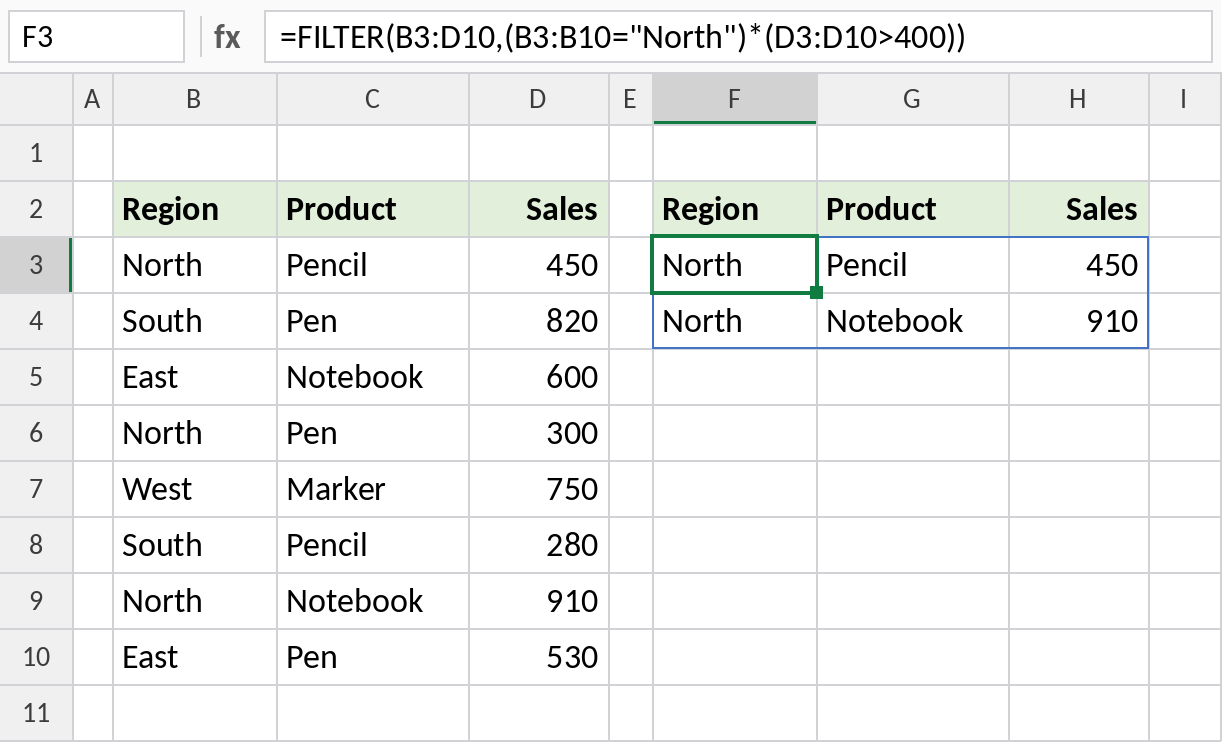

Excel FILTER with two conditions returning North rows with sales over 400

Only North rows with sales above 400 remain: Pencil (450) and Notebook (910). Multiplying works like AND because TRUE × TRUE = 1, and anything with a FALSE becomes 0.

Either condition (OR)

Add the tests instead of multiplying them to keep rows where any test is TRUE:

=FILTER(B3:D10,(B3:B10="East")+(B3:B10="West"))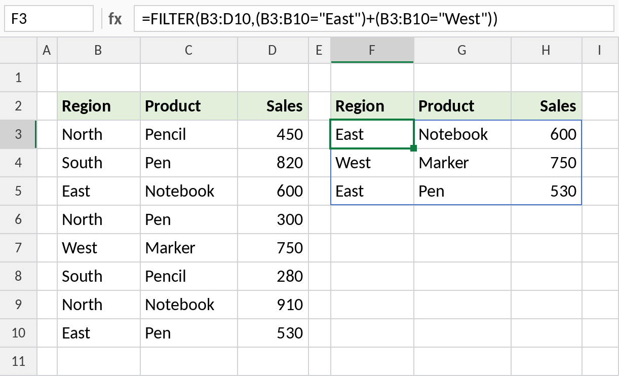

Excel FILTER with OR logic returning East or West rows

All East and West rows are returned, 3 rows in total, in their original order. Adding works like OR because any TRUE makes the sum at least 1.

Show a message when nothing matches

Use the third argument to show a message instead of an error when no rows match:

=FILTER(B3:D10,B3:B10="Central","No results")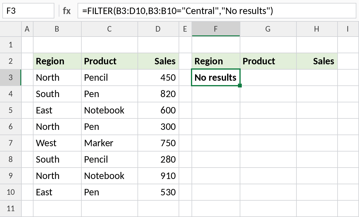

Excel FILTER showing No results when nothing matches

There’s no Central region, so FILTER returns No results instead of #CALC!.

Building the include test

You want	include
Region is North	`B3:B10="North"`
Sales over 500	`D3:D10>500`
North AND over 500	`(B3:B10="North")*(D3:D10>500)`
North OR South	`(B3:B10="North")+(B3:B10="South")`
Product contains “pen”	`ISNUMBER(SEARCH("pen",C3:C10))`
Region matches cell G1	`B3:B10=G1`

Wrap FILTER in SORT to sort the results, or use =ROWS(FILTER(...)) to count them.

Notes

FILTER returns a spill range. Keep the cells below and to the right empty, or you’ll get #SPILL!.
include must be the same height as array.
To refer to the whole result elsewhere, use the spill reference F3#.
If you share files with people on Excel 2019 or earlier, they’ll see #NAME?.

Common errors

Problem	Cause	Fix
`#CALC!`	No rows match and `if_empty` is missing	Add a third argument such as `"No results"`
`#SPILL!`	Cells in the spill range aren’t empty	Clear the cells, or move the formula
`#VALUE!`	`include` is a different height from `array`	Make both ranges cover the same rows
Results don’t include new rows	The ranges stop at row 10	Use an Excel Table, so ranges grow automatically

Practice file

All four examples with working formulas (Excel 2021 or 365).

Download .xlsx