The Excel VLOOKUP function looks for a value in the first column of a table and returns a value from another column in the same row.
lookup_value |
The value to find in the first column of the table. |
|---|---|
table_array |
The table to search. The lookup column must be the first column. |
col_index_num |
Which column of the table to return, counting from 1. |
range_lookup optional |
FALSE for an exact match. TRUE or omitted for an approximate match. |
Table of Contents
Basic example
To find the price of a product from its ID, look it up in the table and return the 4th column. Use FALSE for an exact match:
=VLOOKUP(H3,B3:E8,4,FALSE) 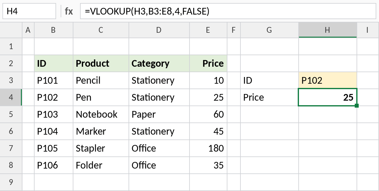
VLOOKUP finds P102 in the first column and returns the value from the 4th column, Price: 25. Always type FALSE for IDs, names and codes.
Approximate match for slabs
With TRUE, VLOOKUP finds the largest value that is less than or equal to the lookup value. This is ideal for discount or tax slabs:
=VLOOKUP(F3,B3:C6,2,TRUE) 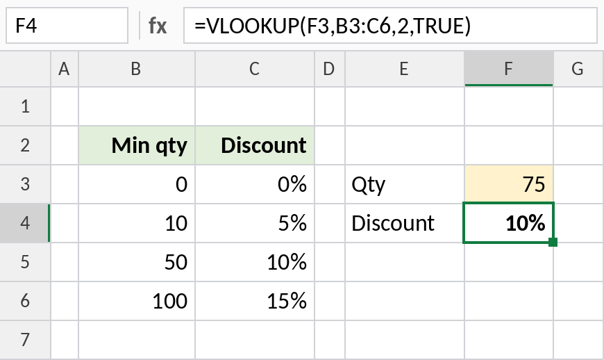
75 isn’t in the table, so VLOOKUP drops back to the slab that starts at 50 and returns 10%. The first column must be sorted smallest to largest for this to work.
Partial match with a wildcard
Join an asterisk to the lookup value to match the start of a text. Here the table starts at the Product column:
=VLOOKUP(H3&"*",C3:E8,3,FALSE) 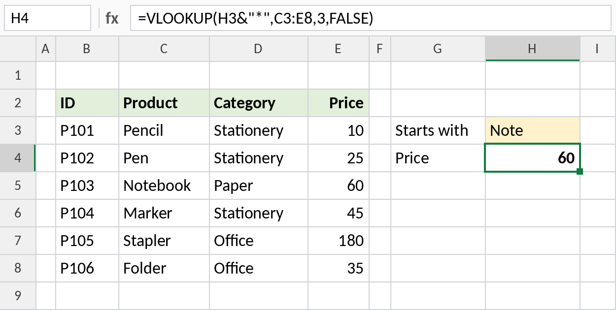
H3&"*" becomes "Note*", which matches Notebook, so VLOOKUP returns its price, 60. Wildcards only work with FALSE.
VLOOKUP limitations
| Limitation | Workaround |
|---|---|
| Can’t return columns to the left | Use XLOOKUP or INDEX and MATCH |
Breaks when columns are inserted, because col_index_num is fixed |
Use MATCH for the column number, or XLOOKUP |
| Approximate match by default | Always type FALSE for exact matches |
| Returns only the first match | Use FILTER for all matches |
Notes
- If you leave out
range_lookup, VLOOKUP uses an approximate match. That’s a common source of wrong results. - VLOOKUP is not case-sensitive.
- Lock the table with
$signs, such as$B$3:$E$8, before filling the formula down. - In Excel 365, XLOOKUP is simpler and more flexible.
Common errors
| Problem | Cause | Fix |
|---|---|---|
#N/A |
The value isn’t in the first column, or extra spaces or numbers stored as text | Check the data, and wrap with IFERROR for a message |
| Wrong value returned | range_lookup left out, so an approximate match was used |
Add FALSE |
#REF! |
col_index_num is larger than the number of columns in the table |
Use a column number inside the table |
| Wrong column after editing | A column was inserted inside the table | Use MATCH for the column number |
Practice file
All three examples plus extra formulas in a cheat sheet.