VLOOKUP and XLOOKUP stop at the first match. To get every order for a customer, use FILTER in Excel 365 and 2021: one formula returns all the matching rows and spills them into the cells below. Here's how, plus a one-cell list with TEXTJOIN and a formula for older versions.
=FILTER(range,condition)All matching rows with FILTER
Type the customer's name in G1 and enter this formula in F4:
=FILTER(A2:D9,B2:B9=G1)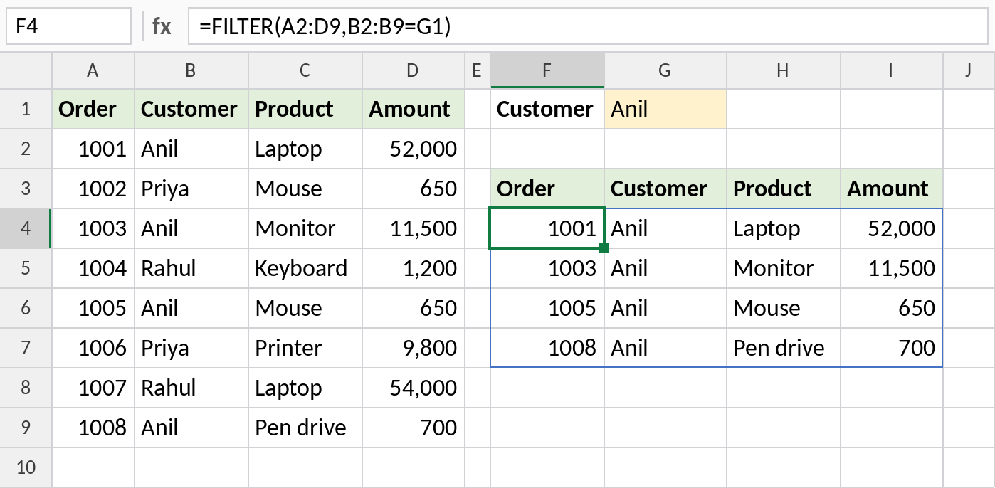
The four rows for Anil spill into F4:I7 (the blue border). Change G1 to Priya and the results resize by themselves. Keep the cells below the formula empty, or you'll get a #SPILL! error.
If nothing matches, FILTER returns #CALC!. Add a message as the 3rd argument: =FILTER(A2:D9,B2:B9=G1,"No orders").
More than one condition
Multiply conditions for AND, and add them for OR:
=FILTER(A2:D9,(B2:B9=G1)*(D2:D9>1000))That returns only Anil's orders above 1,000. (B2:B9="Anil")+(B2:B9="Priya") returns orders for either customer. More in the FILTER function guide.
All matches in one cell
To list a customer's products in a single cell, separated by commas, put FILTER inside TEXTJOIN:
=TEXTJOIN(", ",TRUE,FILTER($C$2:$C$9,$B$2:$B$9=F2))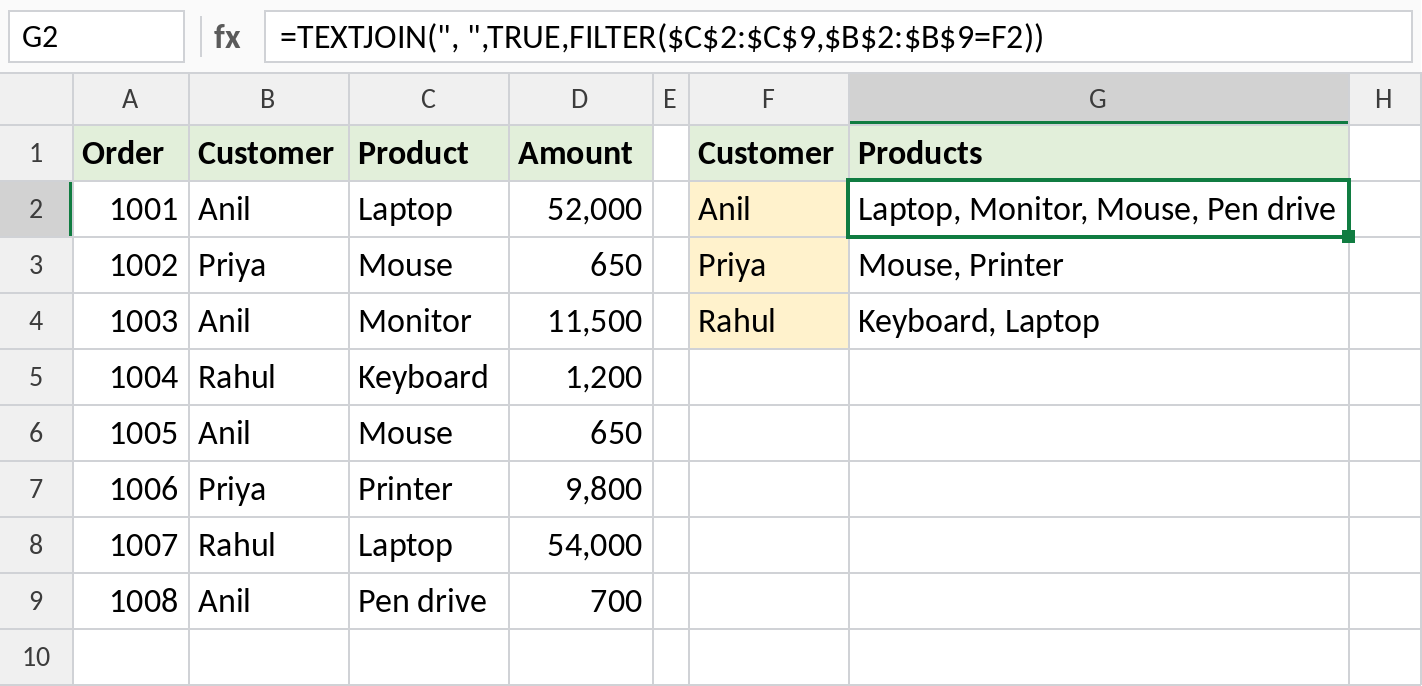
In Excel 2019, which has TEXTJOIN but not FILTER, use IF instead and press Ctrl + Shift + Enter: =TEXTJOIN(", ",TRUE,IF($B$2:$B$9=F2,$C$2:$C$9,"")).
Sort and pick columns
Dynamic array functions can be nested. This returns only the Product and Amount columns for Anil, largest amount first:
=SORT(FILTER(C2:D9,B2:B9=G1),2,-1)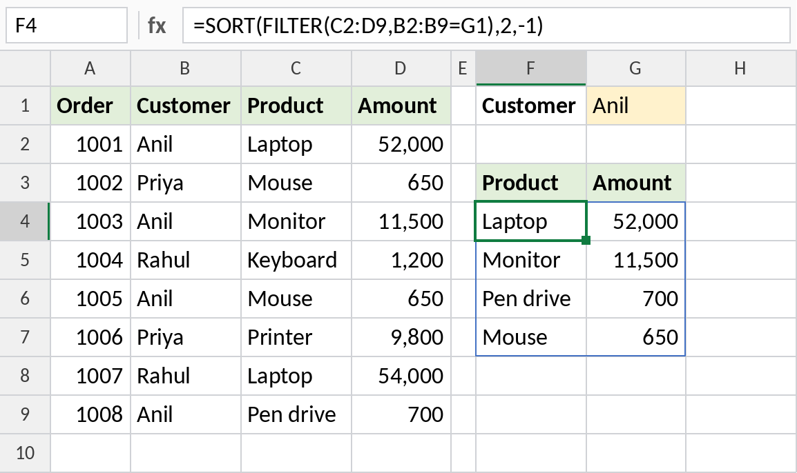
To pick columns that aren't next to each other, use CHOOSECOLS: =CHOOSECOLS(FILTER(A2:D9,B2:B9=G1),3,4).
Other dynamic array lookups
| Goal | Formula |
|---|---|
| A whole row for one match | =XLOOKUP(G1,B2:B9,A2:D9) returns all four columns of the first match |
| Look up a list of values at once | =XLOOKUP(F2:F4,B2:B9,D2:D9) spills one result per value |
| A list of customers to pick from | =UNIQUE(B2:B9), or =SORT(UNIQUE(B2:B9)) |
| How many matches | =COUNTIF(B2:B9,G1) or =ROWS(FILTER(A2:D9,B2:B9=G1)) |
| The last match | =XLOOKUP(G1,B2:B9,C2:C9,,0,-1) |
Learn the whole family in dynamic array functions.
Excel 2019 and older: INDEX and AGGREGATE
Without FILTER, enter this in the first result cell and copy it down as many rows as you might need. It returns the 1st, 2nd, 3rd… match, and a blank when they run out:
=IFERROR(INDEX($C$2:$C$9,AGGREGATE(15,6,(ROW($B$2:$B$9)-ROW($B$2)+1)/($B$2:$B$9=$G$1),ROWS($1:1))),"")($B$2:$B$9=$G$1)is TRUE for Anil's rows. Dividing the row positions by it gives #DIV/0! for every other row.AGGREGATE(15,6,...,k)is SMALL that ignores errors (option 6), so it returns the k-th matching position.ROWS($1:1)becomes 1, 2, 3… as you copy down. INDEX returns the product at each position.
It works in Excel 2010 and later without Ctrl + Shift + Enter. If your file only opens in Excel 365, FILTER is far simpler.
Frequently asked questions
Can VLOOKUP return multiple values?
No. VLOOKUP and XLOOKUP return the first match only. Use FILTER, or the INDEX and AGGREGATE formula in older versions.
Why do I get #SPILL!?
Something is in the cells where the results need to go. Clear them, or move the formula.