#N/A means not available: the lookup function couldn't find the value. Sometimes the value really is missing. Often it is there, but an extra space, a number stored as text or an unlocked range stops it matching. Here's how to find the cause, fix it, and show a friendly message for values that are genuinely missing.
Two #N/A errors, two different reasons
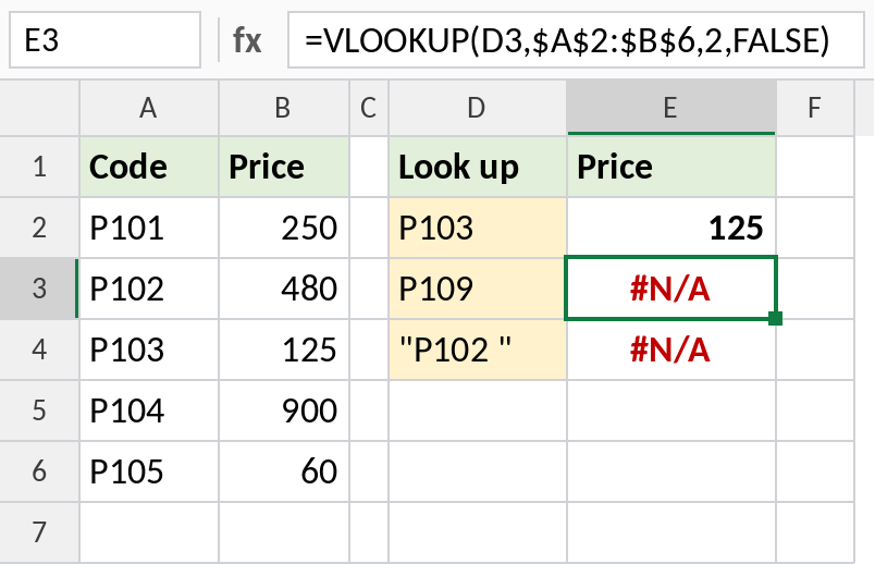
- P109 isn't in the price list. This #N/A is correct.
- P102 has a space at the end (shown in quotes here). P102 is in the list, but P102 with a space isn't, so VLOOKUP returns #N/A.
To check, click the cell and use =LEN(D4): it returns 5 instead of 4. Or test =D4=A3, which returns FALSE.
The fix: TRIM the value, then handle what's still missing
=XLOOKUP(TRIM(D4),$A$2:$A$6,$B$2:$B$6,"Not found")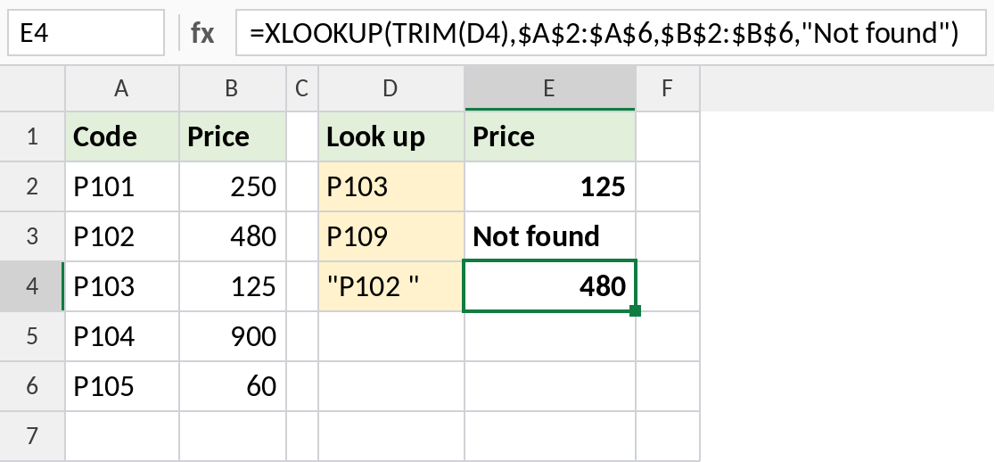
TRIM removes the extra space so P102 is found. XLOOKUP's 4th argument shows Not found for codes that really aren't in the list. With VLOOKUP, wrap it in IFNA instead:
=IFNA(VLOOKUP(TRIM(D4),$A$2:$B$6,2,FALSE),"Not found")If the spaces are in the table rather than the lookup value, clean the table once (TRIM in a helper column, then Paste Values) instead of trimming inside every formula.
Causes of #N/A and how to fix each
| Cause | How to spot it | Fix |
|---|---|---|
| Value really isn't there | Search with Ctrl + F | Show a message with IFNA or if_not_found |
| Extra spaces | =LEN() is longer than expected |
TRIM() |
| Non-breaking spaces from web or ERP data | TRIM doesn't help | SUBSTITUTE(D2,CHAR(160),"") |
| Number stored as text (or the other way round) | Green triangle, or values aligned left | VALUE(D2) or D2&"" to make both sides the same type |
| Range not locked, so it moved when copied | The range shifts in lower rows (A3:B7, A4:B8…) | Add $: $A$2:$B$6 |
| VLOOKUP's value isn't in the first column | The lookup column is to the right of the result | Use INDEX MATCH or XLOOKUP |
| Approximate match, value below the first entry | Only small values fail | Start the table at 0. See exact vs approximate |
Numbers stored as text
1001 the number and "1001" the text look the same, but they don't match. Make the lookup value the same type as the table:
=VLOOKUP(D2&"",$A$2:$B$100,2,FALSE)Use this when the IDs in the table are text and the lookup value is a number. When the table has real numbers and the lookup value is text, use VALUE(D2) instead. To fix the table itself, select the column and use Data → Text to Columns → Finish.
IFNA or IFERROR?
Use IFNA. It replaces only #N/A, so if you also typed a wrong column number (#REF!) or there's text in a number column (#VALUE!), you still see that error. IFERROR hides every error, including real mistakes in the formula.
| Formula | Hides #N/A | Hides #REF!, #VALUE!, #DIV/0! |
|---|---|---|
=IFNA(VLOOKUP(...),"Not found") |
Yes | No |
=IFERROR(VLOOKUP(...),"Not found") |
Yes | Yes |
If the results will be added up, return 0 instead of text: =IFNA(VLOOKUP(...),0).
Frequently asked questions
Why does VLOOKUP return #N/A when I can see the value?
Almost always it's extra spaces, a non-breaking space or a number stored as text. Check with LEN, then use TRIM or VALUE.
How do I return a blank instead of #N/A?
Use =IFNA(VLOOKUP(...),""), or put "" as XLOOKUP's 4th argument.