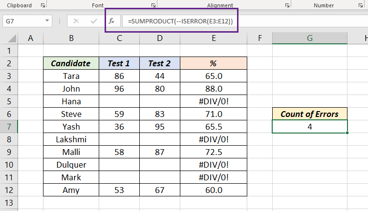
By combining SUMPRODUCT and ISERROR functions in Excel we can find the number of cells containing the Errors.
Table of Contents
Formula
The following formula returns the number of errors in the range E3:E12.
=SUMPRODUCT(--ISERROR(E3:E12))

Explanation
SUMPRODUCT functions multiplies the arrays specified in it and returns the ‘sum of products’ as result. If a single array is used inside it, SUMPRODUCT function will return the sum of values in that array.
ISERROR function returns TRUE if a cell contains an error and FALSE if it doesn’t. Here, when the range E3:E12 is used inside ISERROR function, the expression evaluates to an array of TRUE and FALSE values.
=SUMPRODUCT(--ISERROR(E3:E12))
=SUMPRODUCT(--{FALSE;FALSE;TRUE;FALSE;FALSE;TRUE;FALSE;TRUE;TRUE;FALSE})
These TRUE and FALSE values are then coerced into 1 (Ones) and 0 (Zeros) using ‘– –‘ double negative (also called double unary). The resulting array will be like,
=SUMPRODUCT({0;0;1;0;0;1;0;1;1;0})
Finally, SUMPRODUCT function will return the sum of values in the array, which is 4 in this case.
Formula using SUM funtion
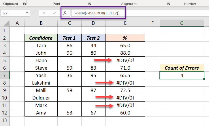
Those whose access to the Dynamic Array Formulas in Excel (which comes with Office 365 Subscription) can use the following formula using SUM function to produce the same result.
=SUM(--ISERROR(E3:E12))
