In this blog post, we will have quick look on the 14 New Functions added to Excel on the 3rd week of March 2022. They are
TEXTSPLIT, TEXTAFTER, TEXTBEFORE, VSTACK, HSTACK, TOROW, TOCOL, WRAPROWS, WRAPCOLS, TAKE, DROP, CHOOSEROWS, CHOOSECOLS, and EXPAND
The first 3 of these new functions TEXTSPLIT, TEXTAFTER, TEXTBEFORE are designed for manipulating text strings.
Table of Contents
TEXTSPLIT
One of the most awaited Excel functions ever, TEXTSPLIT function will split a Text String on the basis of the specified Delimiter.
See how the TEXTSPLIT function splits the given Name into First, Middle, Last Names and spills them into different cells.
=TEXTSPLIT("Christopher Edward Nolan"," ")
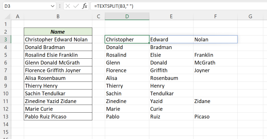
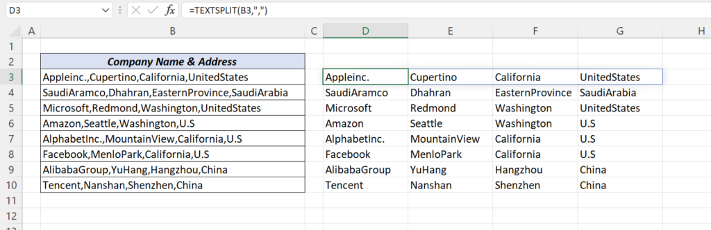
In the above example, ‘Space’ is the delimiter. Following is another example where ‘Comma’ is the delimiter.
=TEXTSPLIT("Appleinc.,Cupertino,California,UnitedStates",",")
Earlier we had to use Text to Columns feature, Power Query or a User Defined Function (UDF) to split text strings. With the new TEXTSPLIT function this task has become a lot more easier and dynamic.
TEXTBEFORE
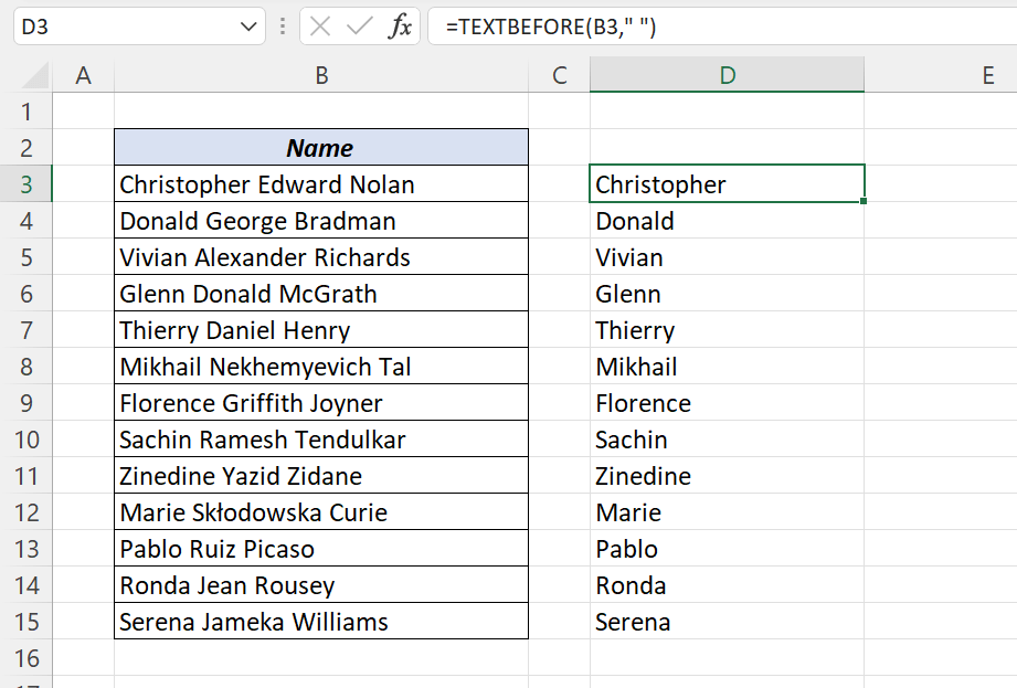
The TEXTBEFORE function can extract all the characters before the specified instance of a particular character or characters.
The following formula will extract Christopher, from Christopher Edward Nolan. i.e., everything before the first ‘Space’ in the supplied string.
=TEXTBEFORE("Christopher Edward Nolan"," ")
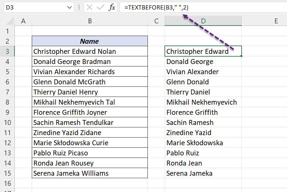
Following formula will extract the First and Middle names. i.e., everything before the second ‘Space’,
=TEXTBEFORE("Christopher Edward Nolan"," ",2)
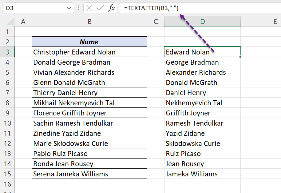
TEXTAFTER
The TEXTAFTER function will return all the characters after the specified instance of a particular character or characters.
The formula given below will extract Edward Nolan, from Christopher Edward Nolan. i.e., everything after the first ‘Space’ in the supplied string.
=TEXTAFTER("Christopher Edward Nolan"," ")
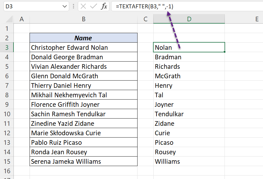
Following formula will extract the Last Name. i.e., everything after the last ‘Space’. The value -1 is used to denote the last instance of the delimiter.
=TEXTAFTER("Christopher Edward Nolan"," ",-1)
Next 2 Functions VSTACK and HSTACK are designed for combining and stacking Arrays.
VSTACK
VSTACK function will stack the supplied arrays vertically.
Following formula will combine the data in the ranges B4:F8, B11:F15, B18:F19 and stack them vertically.
=VSTACK(B4:F8,B11:F15,B18:F19)
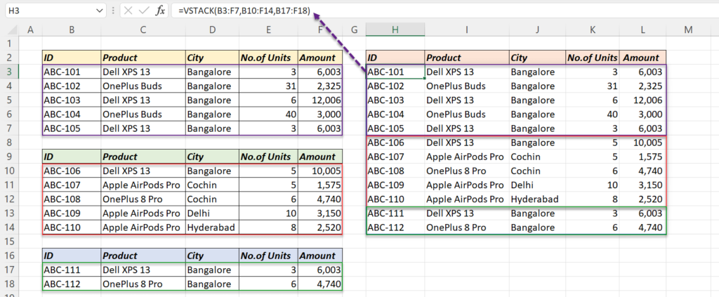
If the source is formatted as an Excel Table, the output will update automatically for the addition of data.
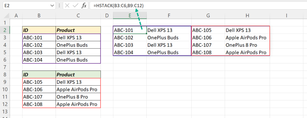
HSTACK
To stack arrays horizontally, we can use the HSTACK function.
Following formula will combine the data in the ranges B3:C6, B9:C12 and stack them vertically.
=HSTACK(B3:C6,B9:C12)
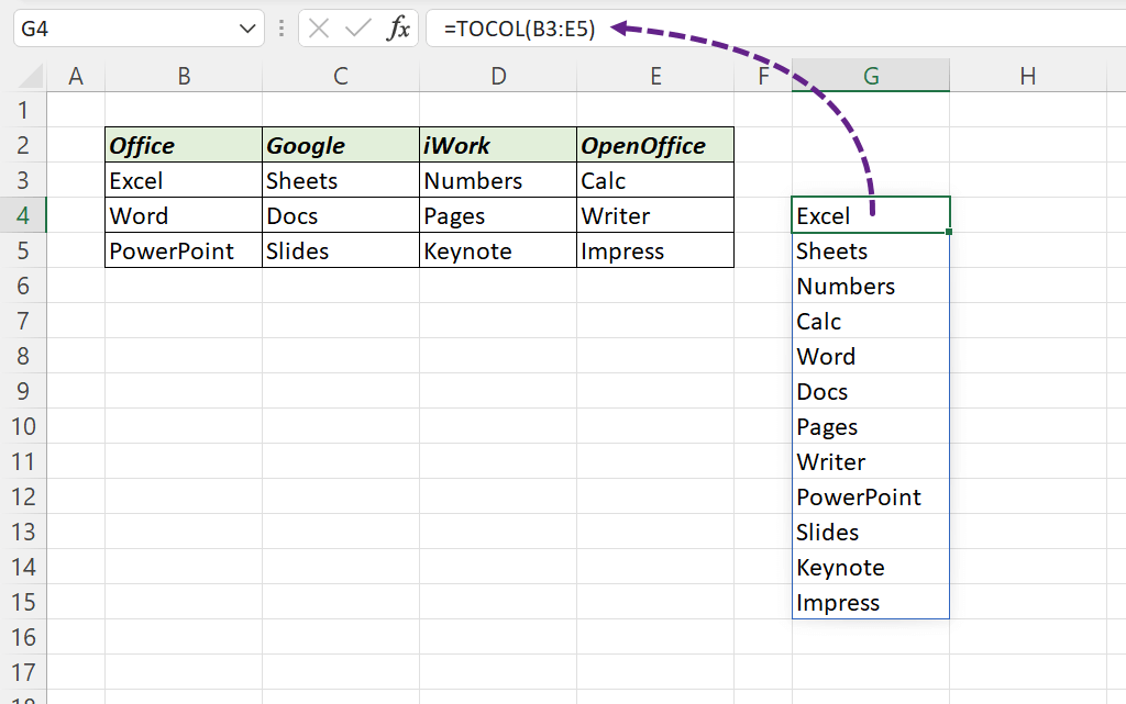
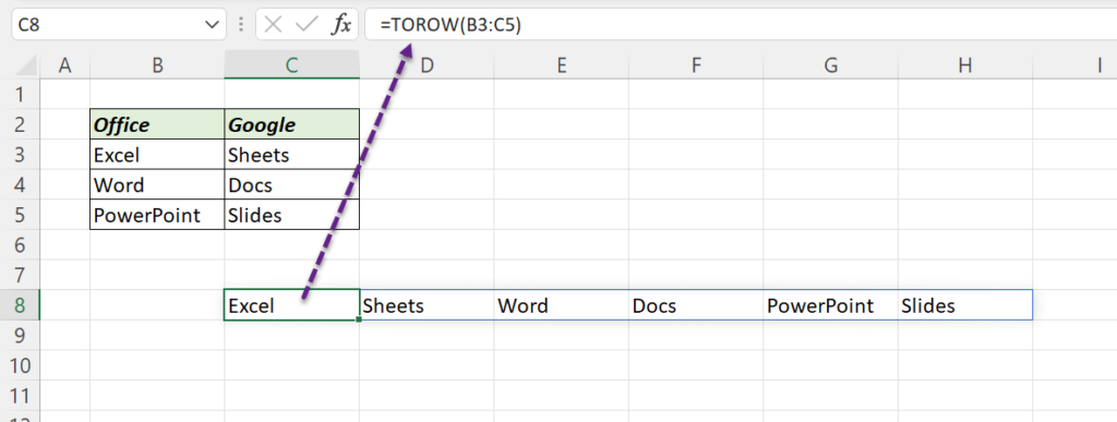
TOCOL and TOROW functions are designed to convert a 2 Dimensional Array into a Single Dimensional Array.
TOCOL
The TOCOL function can be used to arrange the elements of a 2 Dimensional Array into a ‘Single Column’.
TOROW
The TOROW function can arrange the elements of a 2 Dimensional Array into a ‘Single Row’.
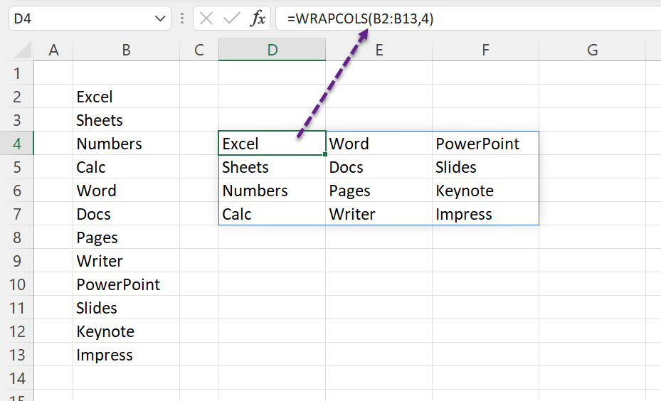
WRAPCOLS and WRAPROWS will do the exact opposite of TOCOL and TOROW functions. These functions are designed to convert a Single Dimensional Array into a Two Dimensional Array of the specified size.
WRAPCOLS
In the following example, WRAPCOLS function converts an Single Dimensional Array of 12 elements into a Two Dimensional Array, where each Column has 4 elements.
=WRAPCOLS(B2:B13,4)
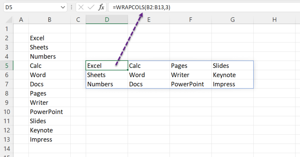
Same Array reshaped into an Array with 3 elements in each Column.
=WRAPCOLS(B2:B13,3)
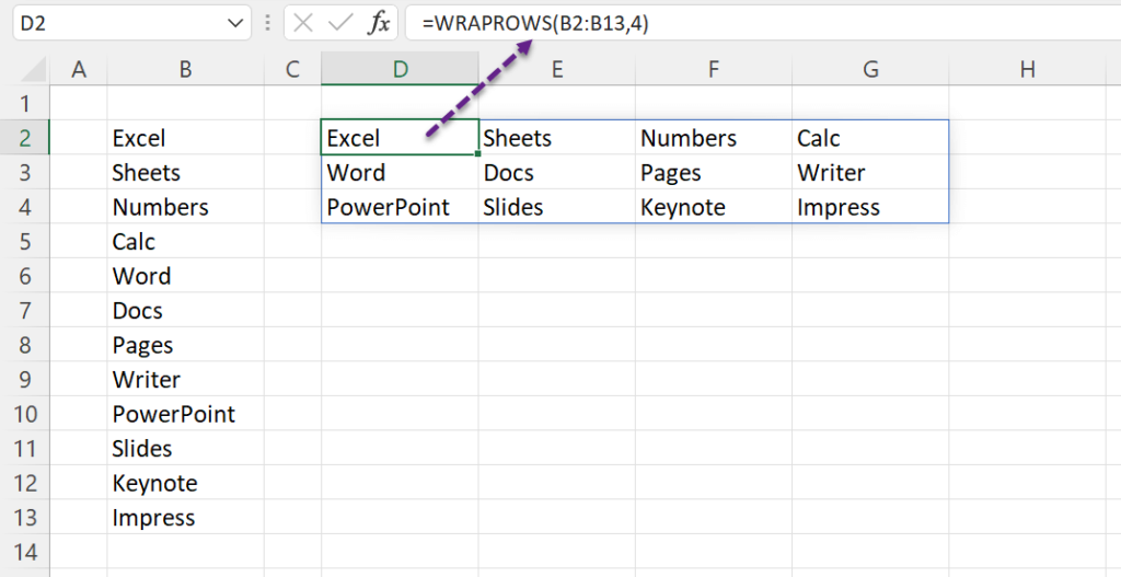
WRAPROWS
In the following example, WRAPROWS function converts an Single Dimensional Array of 12 elements into a Two Dimensional Array, where each Row will have 4 elements.
=WRAPROWS(B2:B13,4)
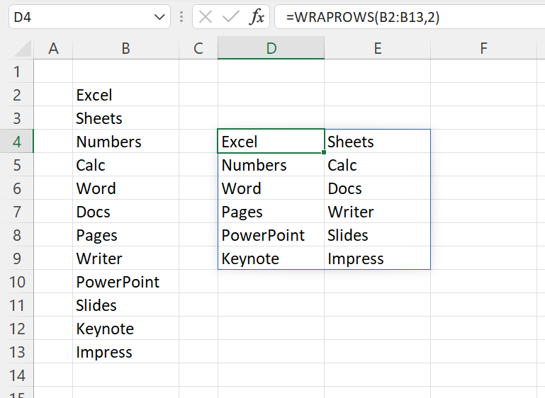
Same Array reshaped into an Array 2 elements in each Row.
=WRAPROWS(B2:B13,2)
Next 5 functions TAKE, DROP, CHOOSECOL, CHOOSEROW and EXPAND are designed to ‘Resize’ Arrays.
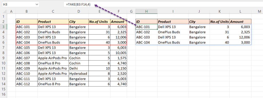
TAKE
TAKE function will return the specified number of Rows and Columns from the start or end of the supplied Array.
Following formula will keep the first 3 rows from the range B3:F14
=TAKE(B3:F14,4)
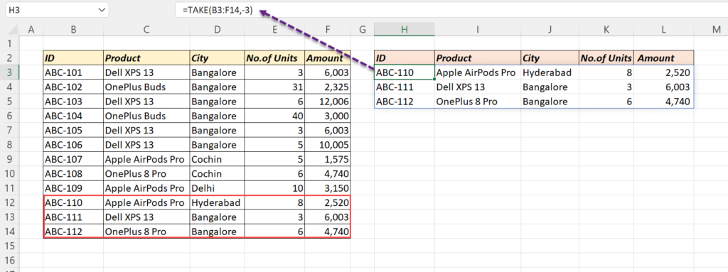
For the last 3 rows from the range B3:F14
=TAKE(B3:F14,-3)
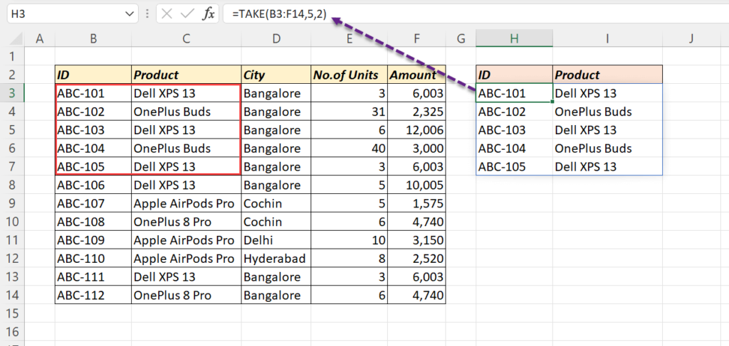
For the first 5 rows and 2 columns from the range B3:F14
=TAKE(B3:F14,5,2)
DROP
The DROP function will drop the specified number of Rows and Columns from the supplied array.
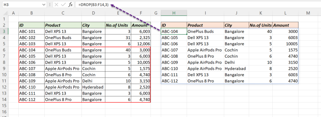
Following formula will drop the first 3 rows from the range B3:F14
=DROP(B3:F14,3)
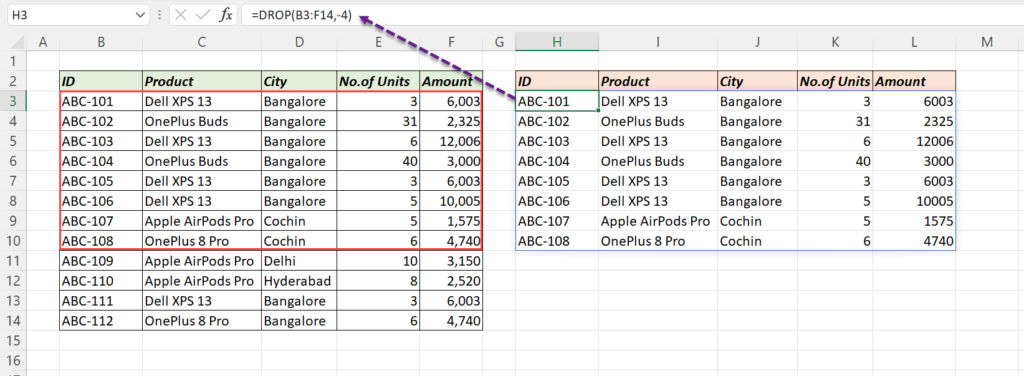
To drop the last 3 rows from the range B3:F14
=DROP(B3:F14,-4)
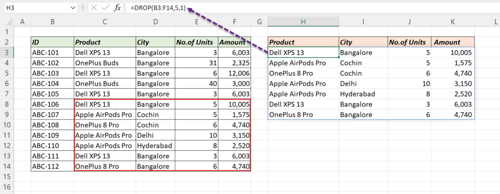
To drop the first 5 rows and 1 column from the range B3:F14
=DROP(B3:F14,5,1)
CHOOSECOLS
CHOOSECOLS will return the specified Columns from the supplied array.
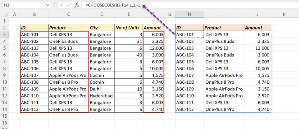
To extract the 1st, 2nd and last columns from the range B3:F14,
=CHOOSECOLS(B3:F14,1,2,-1)
CHOOSEROWS
To extract the specified Rows from the supplied array, we can use the CHOOSEROWS function.
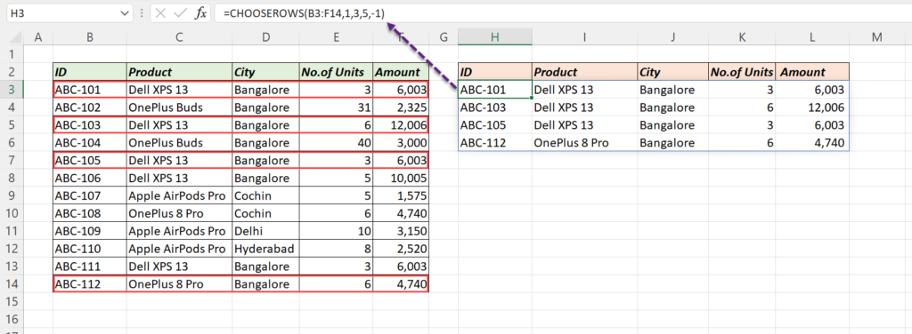
The following formula will return the 1st, 3rd, 5th and last Rows from the range B3;F14.
=CHOOSEROWS(B3:F14,1,3,5,-1)
EXPAND
The EXPAND function will expand an Array into the specified dimensions.
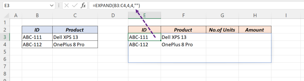
The following formula expands a 2 x 2 size Array into a 4 x 4 size Array.
=EXPAND(B3:C4,4,4,"")
While expanding the Array with the EXPAND function, we can decide what is to be filled in the blank spaces. Here, I have used ‘Space’ character.
Why EXPAND function?
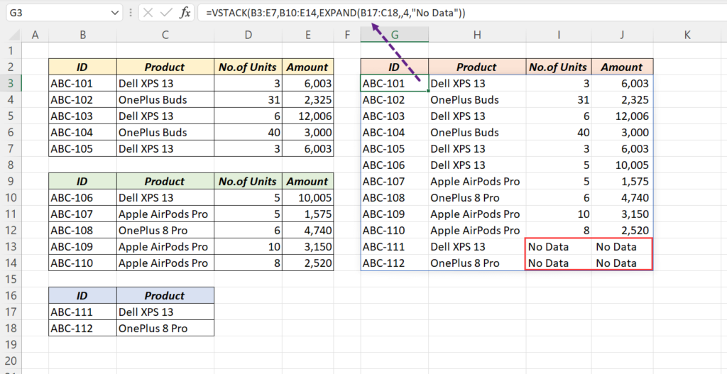
In the following scenario, VSTACK function is used to combine 3 Arrays of different sizes.
=VSTACK(B3:E5,B9:E13,B16:C17)
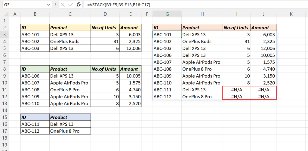
Due to the different sizes of Arrays, the final Array have some #N/A Errors.
These Errors can be replaced with a Custom Value by resizing the supplied Arrays using the EXPAND function.
=VSTACK(B3:E7,B10:E14,EXPAND(B17:C18,,4,"No Data"))
At this point of Time, these functions are only available to users running Beta Channel of Office Insiders.
Version 2203 (Build 15104.20004) or later on Windows and Version 16.60 (Build 22030400) or later on Mac.