By combining the SUMPRODUCT and YEAR functions in Excel we can find the number of Dates in a given Year.
Table of Contents
Formula
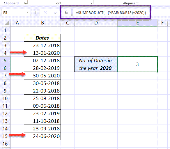
Here we have a list of dates in the cells from B3:B15. The following formula will return the number of dates in the year 2020.
=SUMPRODUCT(--(YEAR(B3:B15)=2020))

Explanation
SUMPRODUCT functions multiplies the arrays specified in it and returns the ‘sum of products’ as result. If a single array is used inside it, SUMPRODUCT function will return the sum of values in that array.
YEAR function extracts the year from a valid Excel date. Here, when the range B3:B15 is used inside YEAR function, the expression evaluates to an array of years like the following.
=SUMPRODUCT(--(YEAR(B3:B15)=2020))
becomes...
=SUMPRODUCT(--({2018;2020;2018;2019;2020;2018;2018;2018;2018;2019;2018;2018;2020}=2020))
Then each of these values will be compared with the value 2020 and produce an array of TRUE and FALSE values.
=SUMPRODUCT(--({FALSE;TRUE;FALSE;FALSE;TRUE;FALSE;FALSE;FALSE;FALSE;FALSE;FALSE;FALSE;TRUE}))
These TRUE and FALSE values are then coerced into 1 (Ones) and 0 (Zeros) using ‘ – –‘ double negative (also called double unary). The resulting array will be like,
=SUMPRODUCT({0;1;0;0;1;0;0;0;0;0;0;0;1})
Finally, SUMPRODUCT function will return the sum of values in the array, which is 3 in this case.
Formula with cell reference
In the above example we were using the direct value ‘2020’. Instead of hard coding the value in the formula, we can use the address of the cell that contains the Year to search for.
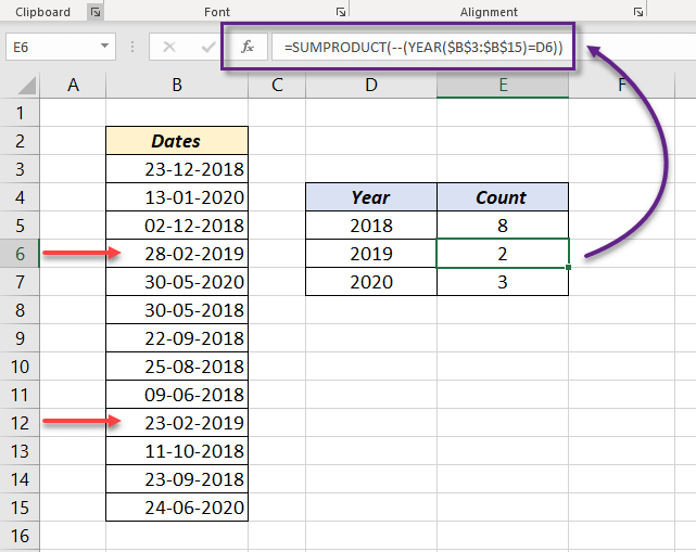
The following formula returns the number of cells containing the date of the Year present in cell D6.
=SUMPRODUCT(--(YEAR($B$3:$B$15)=D6))
Here, the cell D6 contains the year ‘2019‘. So the formula returned the value 2.
