An exact match returns a result only when the lookup value is found exactly. An approximate match returns the nearest value below it, which is what you need for grade bands, tax slabs and commission rates. Using the wrong one is the most common reason a lookup returns a wrong answer without showing any error.
Approximate match: grades from marks
The grade table lists the lowest mark for each grade, sorted smallest to largest. With TRUE as the last argument, VLOOKUP finds the largest minimum mark that is not more than the student's marks:
=VLOOKUP(E2,$A$2:$B$7,2,TRUE)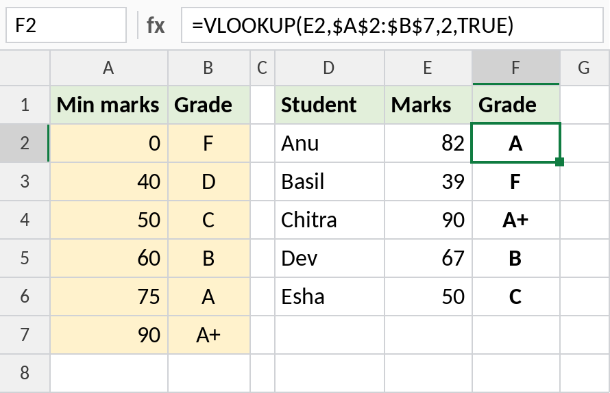
- 82 isn't in the table. The largest value not above 82 is 75, so the grade is A.
- 90 is in the table, so it gets A+. An exact hit is used when there is one.
- 39 falls between 0 and 40, so it gets F.
The same thing with XLOOKUP
In XLOOKUP, the 5th argument -1 means exact match or next smaller item. The table doesn't need to be sorted:
=XLOOKUP(E2,$A$2:$A$7,$B$2:$B$7,,-1)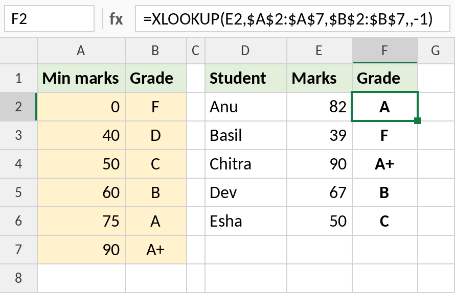
Use 1 instead for exact match or next larger item. For example, pick the smallest box size that fits a parcel, or the next pricing tier up.
Match types in each lookup function
| Function | Exact match | Next smaller | Next larger | Needs sorting? |
|---|---|---|---|---|
| VLOOKUP, HLOOKUP | FALSE or 0 |
TRUE, 1 or left out |
Not available | Yes, ascending, for approximate |
| MATCH | 0 |
1 or left out |
-1 |
Ascending for 1, descending for -1 |
| XLOOKUP, XMATCH | 0 or left out |
-1 |
1 |
No |
| LOOKUP | Not available | Always | Not available | Yes, ascending |
XLOOKUP and XMATCH are the safe choice: exact by default, and their approximate modes work on unsorted lists.
The trap: a missing FALSE in VLOOKUP
=VLOOKUP(D2,A2:B100,2) has no 4th argument, so it does an approximate match. On a list of codes or IDs that isn't sorted, it can return the price of a different product, with no error to warn you. Always finish VLOOKUP with FALSE (or 0) unless you really want a band lookup:
=VLOOKUP(D2,A2:B100,2,FALSE)The same goes for MATCH: always type the 0 for an exact match.
Rules for approximate match tables
- Put the lowest value of each band in the first column, not a range like 40-49.
- Start the table at the lowest possible value (0 for marks). A lookup value below the first entry returns #N/A.
- Sort the first column smallest to largest for VLOOKUP, MATCH and LOOKUP.
- Lock the table with
$signs before copying the formula down.
Other kinds of match
- Wildcards:
*matches any text and?matches one character.=VLOOKUP("Raj*",A2:B8,2,FALSE)finds the first name starting with Raj. In XLOOKUP, set the match mode to2. - Case: all lookups ignore case, so anil matches ANIL. For a case-sensitive lookup use
=XLOOKUP(TRUE,EXACT(A2:A8,D2),B2:B8). - Last match: XLOOKUP's 6th argument
-1searches from the bottom up.
Frequently asked questions
Why does my VLOOKUP return a wrong value instead of #N/A?
The 4th argument is missing or TRUE, so it's doing an approximate match on a list that isn't sorted. Add FALSE.
Is TRUE the same as 1 in VLOOKUP?
Yes. TRUE and 1 both mean approximate match, and FALSE and 0 both mean exact match.