INDEX MATCH is two functions working together. MATCH finds the row number of the value you want, and INDEX returns the value from that row in any column. It looks left as well as right, and it doesn't break when you insert a column. It works in every version of Excel.
INDEX(result, MATCH(value, list, 0))The basic INDEX MATCH formula
The employee list is in A1:E8. To get the salary for the Emp ID in H2:
=INDEX(E2:E8,MATCH(H2,A2:A8,0))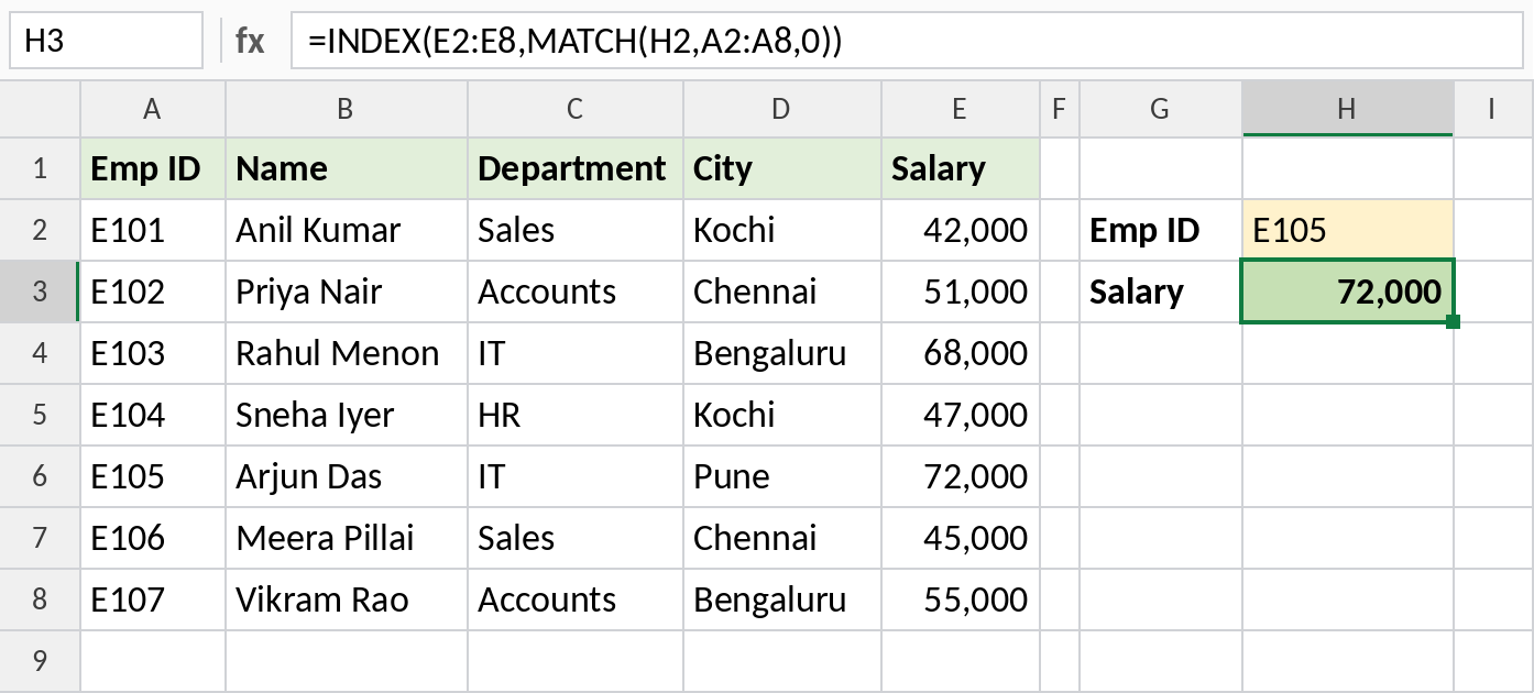
MATCH(H2,A2:A8,0)looks for E105 in A2:A8 and returns 5, because it's the 5th item. The0means exact match.INDEX(E2:E8,5)returns the 5th value in E2:E8: 72,000.
Keep the two ranges the same size and starting on the same row (here both run from row 2 to row 8). If they don't line up, you get the wrong row's value without any error.
Look up to the left
VLOOKUP can only return columns to the right of the lookup column. INDEX MATCH doesn't care. Here the name is in column B and the Emp ID we want is in column A, to its left:
=INDEX(A2:A8,MATCH(H2,B2:B8,0))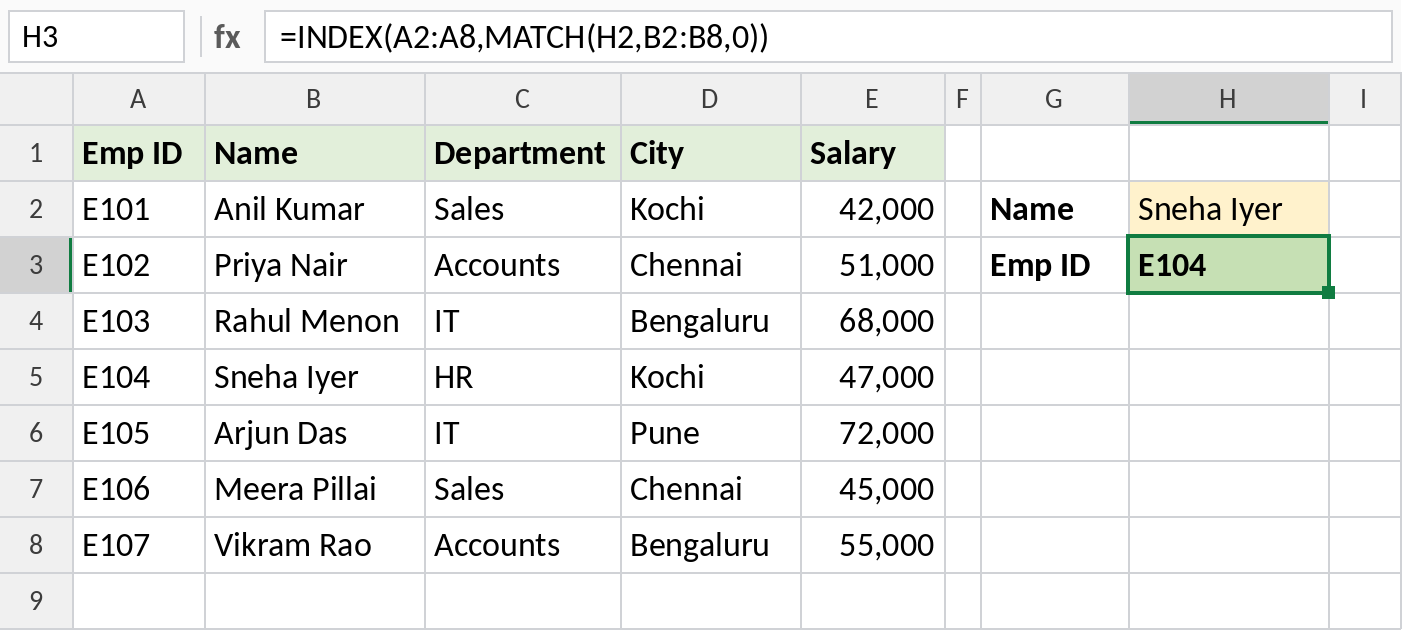
Two-way lookup: match the row and the column
INDEX accepts a row number and a column number. Use one MATCH for each, and the field you return can be chosen from a cell:
=INDEX(A2:E8,MATCH(H2,A2:A8,0),MATCH(H3,A1:E1,0))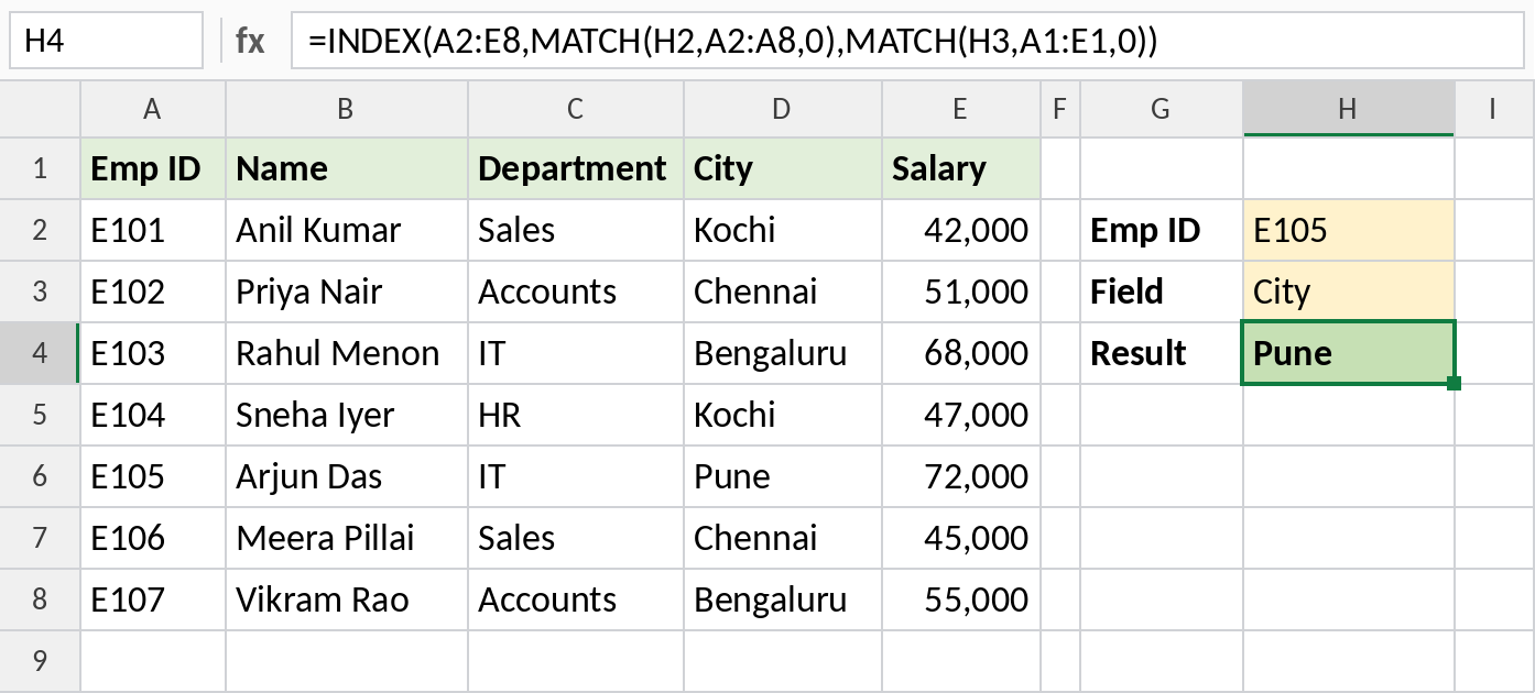
Type Salary or Department in H3 and the result changes. More examples in two-way lookup in Excel.
INDEX MATCH with multiple criteria
To find the salary of the person in the IT department in Pune, multiply the two tests. Each row becomes 1 only when both are TRUE, and MATCH looks for that 1:
=INDEX(E2:E8,MATCH(1,(C2:C8=H2)*(D2:D8=H3),0))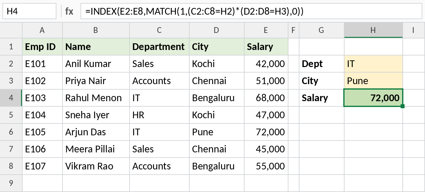
In Excel 365 and 2021, press Enter. In Excel 2019 and older, press Ctrl + Shift + Enter. More methods in VLOOKUP with multiple criteria.
Approximate match with INDEX MATCH
Change the last argument of MATCH to 1 to find the largest value that is less than or equal to the lookup value, for tax slabs, grades and commission bands. The lookup range must be sorted smallest to largest:
=INDEX(B2:B7,MATCH(E2,A2:A7,1))See exact vs approximate match for how it works.
INDEX MATCH vs VLOOKUP vs XLOOKUP
| VLOOKUP | INDEX MATCH | XLOOKUP | |
|---|---|---|---|
| Look to the left | No | Yes | Yes |
| Insert a column in the table | Can return the wrong column | Keeps working | Keeps working |
| Default match | Approximate (if you leave out FALSE) | Approximate (if you leave out 0) | Exact |
| Message when not found | Wrap in IFNA | Wrap in IFNA | Built in |
| Excel versions | All | All | Excel 2021 and 365 |
If everyone who opens your file has Excel 2021 or 365, use XLOOKUP. It does all of this in one function. Use INDEX MATCH when the file must work in Excel 2019 or older. See XLOOKUP vs VLOOKUP.
Common errors
| Error | Usual cause | Fix |
|---|---|---|
| #N/A | The value isn't in the lookup range, or has extra spaces | See fix #N/A errors |
| #REF! | The row or column number is bigger than the INDEX range | Make the INDEX range match the MATCH range |
| Wrong value, no error | MATCH has no 0, or the two ranges start on different rows |
Add ,0 and line up the ranges |
Frequently asked questions
Is INDEX MATCH faster than VLOOKUP?
On normal-sized sheets you won't notice a difference. The real advantages are looking left and not breaking when columns are added.
Should I still learn INDEX MATCH if I have XLOOKUP?
Yes. You'll meet it in files made by other people, it works in every version, and INDEX and MATCH are useful on their own.