When we transform data using Power Query, every Transformation Step is recorded as an M Code. And most of the time, values got hard coded in these codes.
The problem with Hard coding is, when the user decides to change the input data, the Source code (Query in this case) also should be modified accordingly.
In this post, I will explain ‘How to introduce Parameters (Variables) within queries and make them more Dynamic’
My friends know my taste for Excel as well as Movies. So, one of my moviegoer friends asked me for the list of 15 Highest Grossing Hollywood Movies of 2010.
In a couple of minutes, I created an Excel sheet using Power Query and sent it to him. Following is the same excel worksheet which I made for him and as you can see, it has much more than what he asked for. The list of Top 5, 10, 15 or any number movies of any year between the 1977 to 2019 is available in this worksheet.
and here is How I did that…
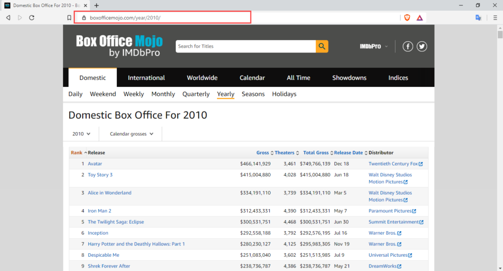
First of all, visit the website of Box Office Mojo and copy the link to the following page which contains the entire list of movies released in 2010.
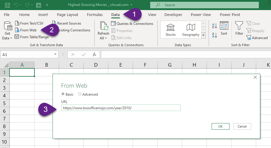
Open an Excel workbook > In the Data of the Excel Ribbon > From Web > Paste the copied link into the From Web dialog > Click OK
There is a dialog called Access Web content asking permission to connect with the website of Box Office Mojo
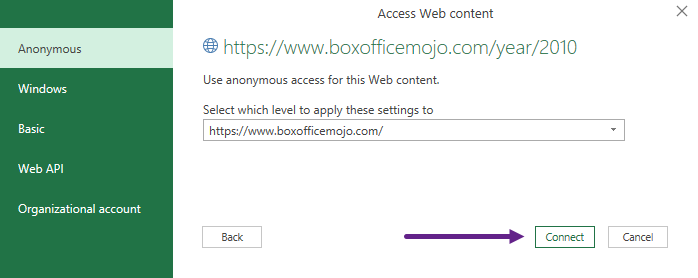
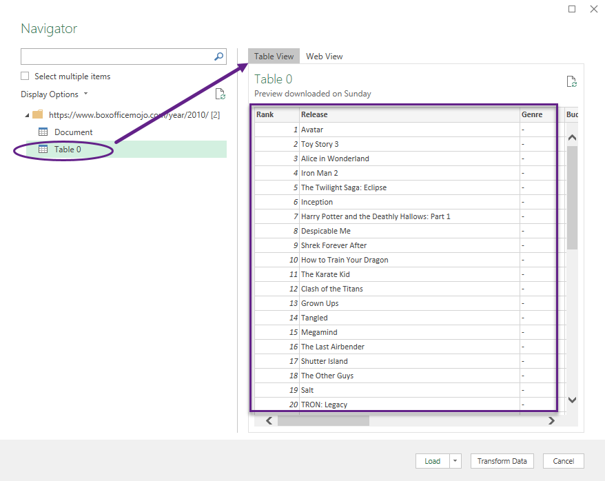
Click on Connect and we will get another dialog called Navigator.
In this dialog there are ‘two items’ listed on the left side bar with their Table View and Web View on right side. After selecting ‘Table 0’ which contains the list of movies, Click on Transform Data
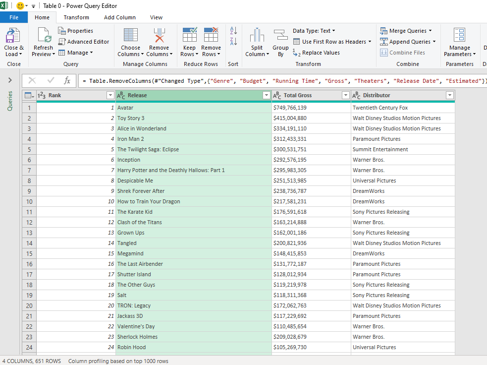
The 651 movies listed in the connected web page are loaded into the Power Query Editor.
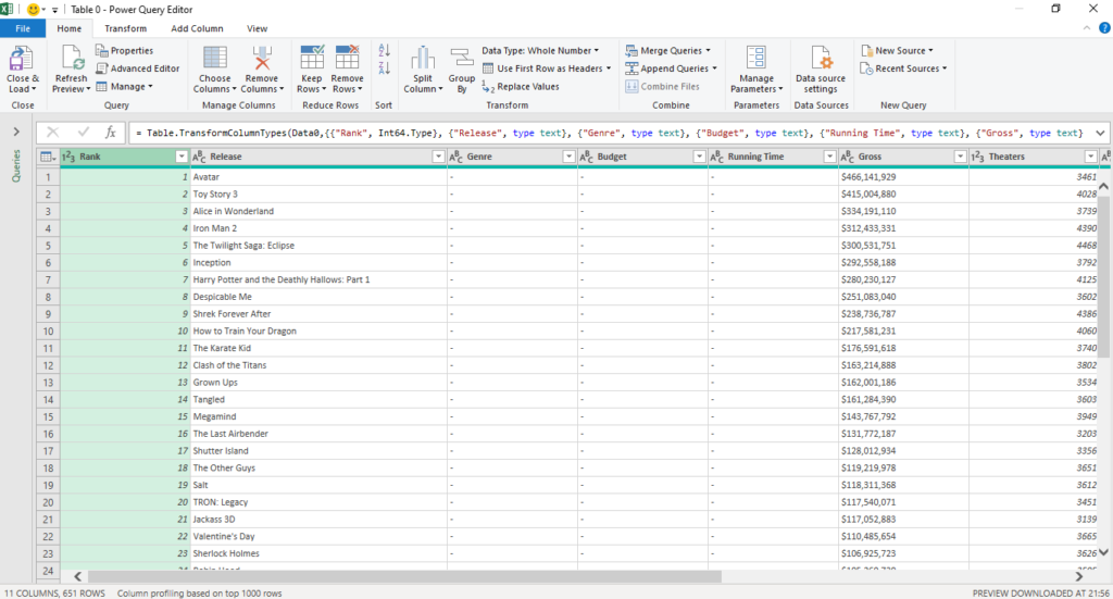
Data Pane shows 11 columns of data, but I need only 4 from these. The columns for ‘Rank’, ‘Movie Name’, ‘Total Gross Collection’ and ‘Distributor’.
To remove the unwanted columns, Select the required columns (holding the CTRL key), right-click on the column header, Select Remove Other Columns.
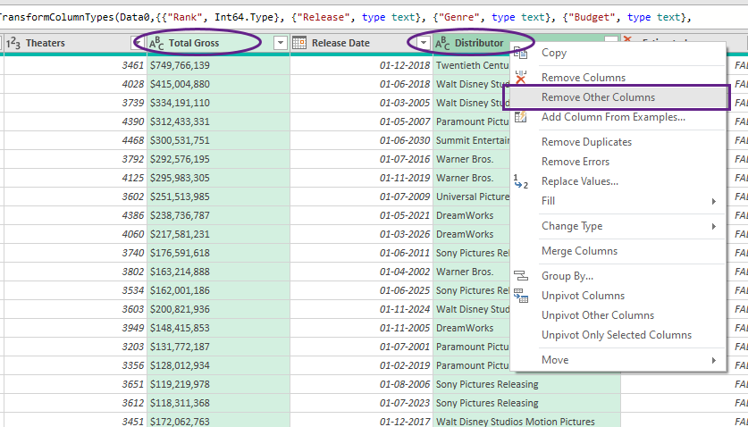
All unwanted columns, except the 4 selected columns are gone.
To remove the rows, except the first 15,
In the Home Tab > Keep Rows > Keep Top Rows > Type in 15 in the input box for Number of Rows > Click OK
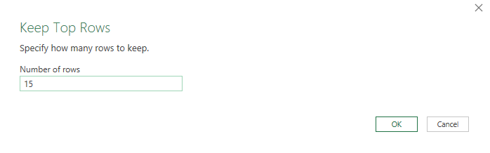
We have the list of the 15 Highest Grossing Movies of 2010.
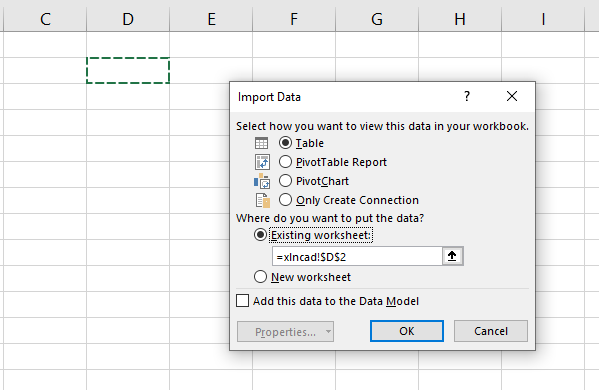
To load this data into an Excel worksheet,
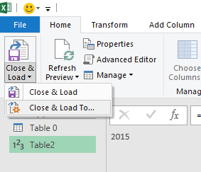
Click on the split button for Close & Load > Close & Load To…
Import Data Dialog will be activated.
In the Import Data dialog, Select Existing worksheet > Select the cell where you want to place the Transformed Data (Here, I have selected the cell D2) > Click OK
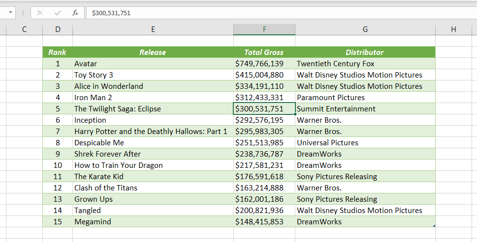
And the following is the data which my friend has asked for, the list of 15 Highest Grossing Hollywood movies of 2010.
I could have send this report to him thinking that he should be happy with this.
But, what if he asks again for the list of 2015 or 2016? Shall I repeat these steps again?
If so, that is going to be a waste of Time as well as Effort. So, I decided to make this report dynamic using the Passing Parameter method in Power Query.
Let’s see how I did that…
Create a One-Dimensional Table with the text Year as heading and the number representing any valid year as it’s content.
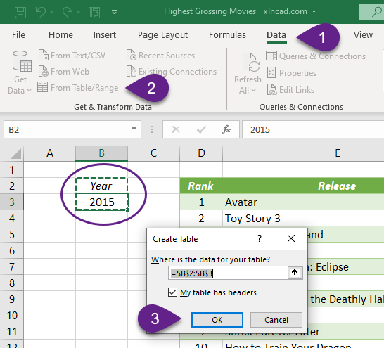
Type in the text Year into the cell B2 and the number 2015 into the cell B3.
To create a Parameter (Query) using this table,
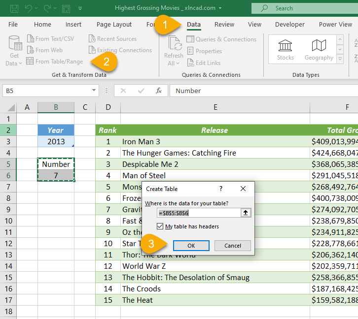
Select a cell in the Table > In the Data tab > From Table/Range > Click OK in the Create Table Dialog
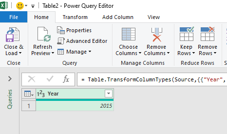
The selected table is loaded into the Power Query Editor.
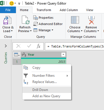
To convert this query into a Parameter, Right-Click on the value > Select Drill Down
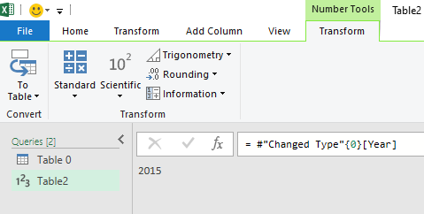
Now the query called Table2 has been converted into a Parameter
To use this parameter inside the first query called Table 0,
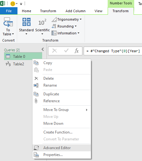
Right-click on Table 0 in the Queries pane and select Advanced Editor
Advanced Editor is activated and following is the M Code of the first query called Table 0
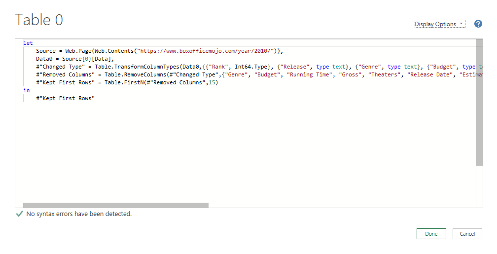
As you can see the year 2010 is hard coded in the link.
Replace 2010 with “&Text.From(Table2)&” in the first statement and the code will look the following

Text.From is a M Function used to convert any kind of value (Number, Date, Time etc.) into text.
Table2 is the Parameter which we created
Source = Web.Page(Web.Contents("https://www.boxofficemojo.com/year/2010/")),

in the M Code was modified to

Source = Web.Page(Web.Contents("https://www.boxofficemojo.com/year/"&Text.From(Table2)&"/")),
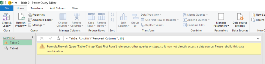
When you close the Advanced Editor, most probably you will get an error like the following. But there is nothing to worry!
This error is a result of Data Privacy Firewall and can be fixed easily.
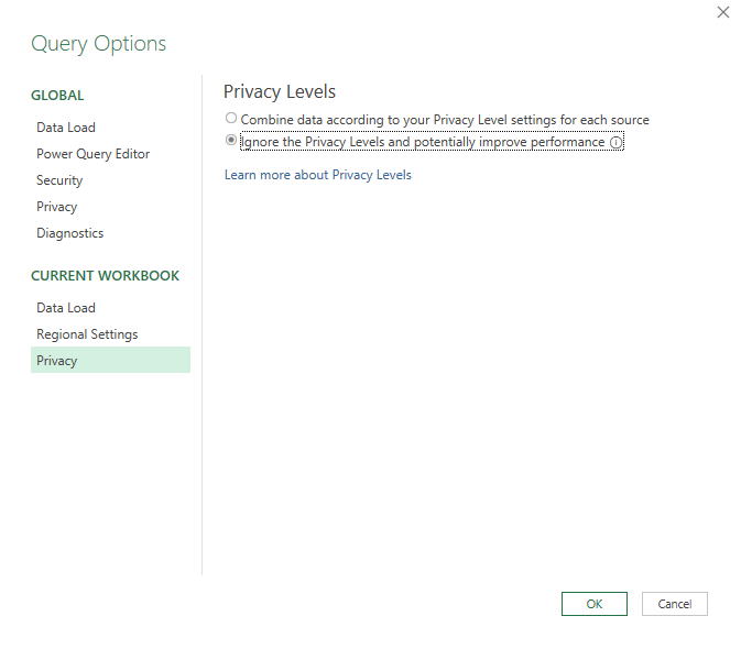
Go to File Tab > Options and Settings > Query Options > Select Privacy under CURRENT WORKBOOK in the left side bar > Select the radio button for Ignore the Privacy Levels and potentially improve performance > Click OK
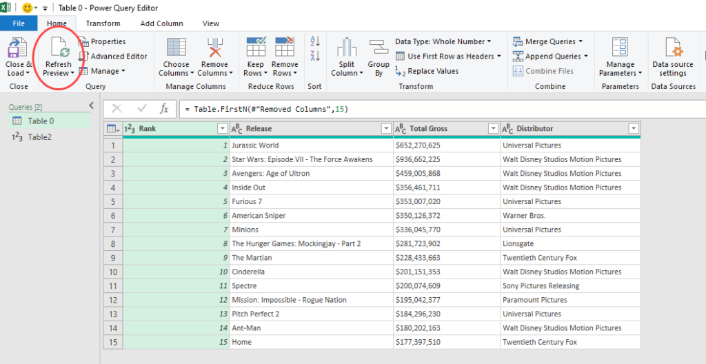
Click on the Refresh Preview in the Home tab and you will see the updated table. i.e. the list of movies for 2015. Please note that the parameter we created holds the value 2015 at this moment and hence the table contains the list of movies from the year 2015.
To save this newly created Parameter (Table2), we will load this query as a Connection. For that,
In the Home tab > Close & Load > Close & Load To…
In the Import Data dialog, select Only Create Connection and Click OK

Now type in any year into the Table for Year and Click on Refresh All in the Data tab to update the list of movies.
Now the worksheet is dynamic and can fetch the list of 15 Highest grossing movies from any year between 1977 and 2019.
but what if he changes his mind and asks for a list of Top 20 movies or Top 30 movies?
So, let’s create another parameter which will help us to decide the number of movies in the list.
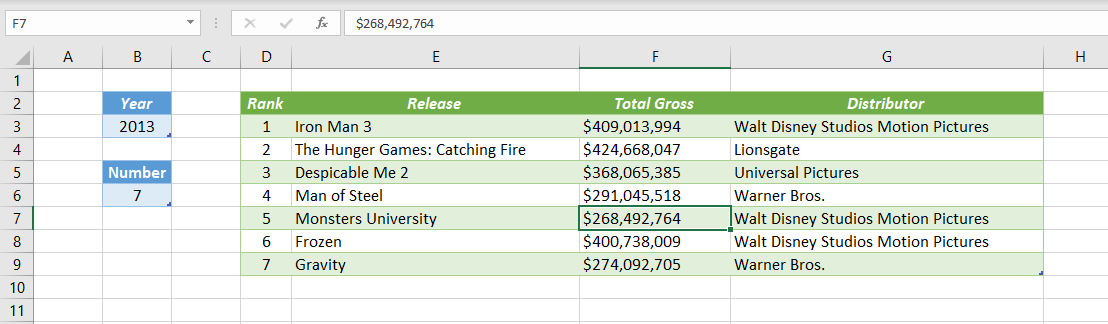
Type in the text Number into the cell B5 and the value 7 (can be any number) into the cell B6.
To create a Parameter (Query) using this table,
Select a cell in the table > In the Data tab > From Table/Range > Click OK in the Create Table Dialog
Selected data is loaded into the Power Query Editor as Table3
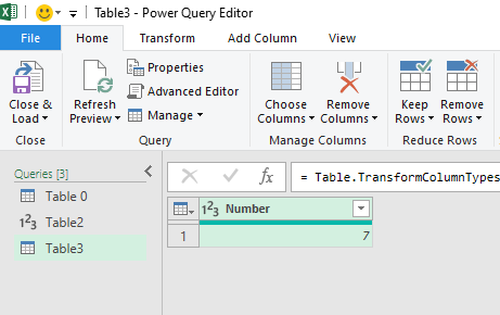
To convert this query into a parameter, Right-Click on the value > Select Drill Down
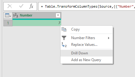
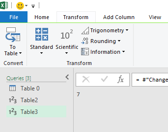
Now the query called Table3 has been converted into a Parameter which holds the value 7.
To use this parameter inside the first query called Table 0, Right-click on Table 0 in the Queries pane and open the Advanced Editor
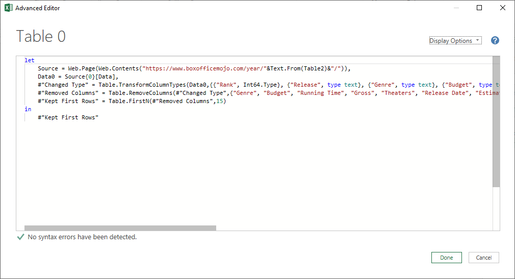
Using the Advanced Editor we will modify the 5th statement in the M Code, which corresponds to Transformation step for removing all rows, except the first 15.
Replace the value 15 with Table3 in the 5th statement of the M Code and the code will look like the following.
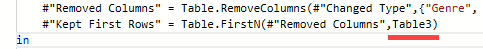
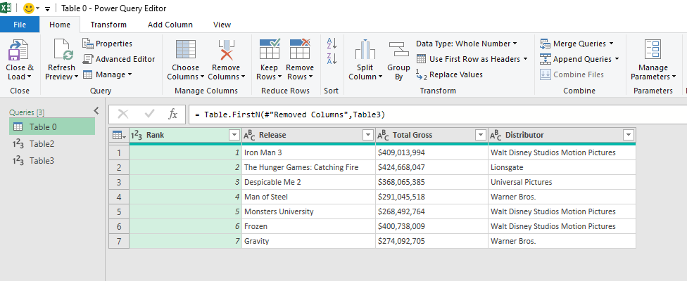
"Kept First Rows" = Table.FirstN(#"Removed Columns",15)

in the M Code was modified to

"Kept First Rows" = Table.FirstN(#"Removed Columns",Table3)
Click on Done and select Table0 from the Queries pane. The table will be updated like the following.
To save this newly created Parameter (Table3), we will load this query as a connection. For that,
Select the Query called Table3 > in the Home tab > Close & Load > Close & Load To… > In the Import Data Dialog > select Only Create Connection
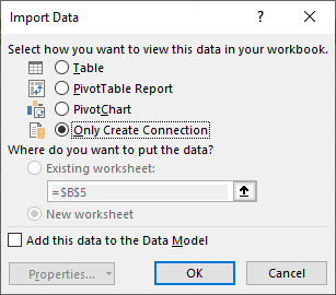
Once when I click OK I have the list of the Top 7 movies of 2013.
Now this worksheet can fetch the Top ‘n’ number of Hollywood films from the year 1977 to 2019. You just need to enter the Year and the value for n into the corresponding tables and Click on Refresh All in the Data tab of Excel Ribbon.

Watch my Video on 12 Methods to Clean Data using Power Query