In the previous post, I have explained How to Combine Data from Multiple Worksheets of an Excel Workbook. That was a crude method of static nature and won’t be the right choice, when you have plans to Add or Delete worksheets.
The method explained here is recommended for those who want to Combine data from Multiple Worksheets of a Workbook and also expects Addition of New Worksheets.
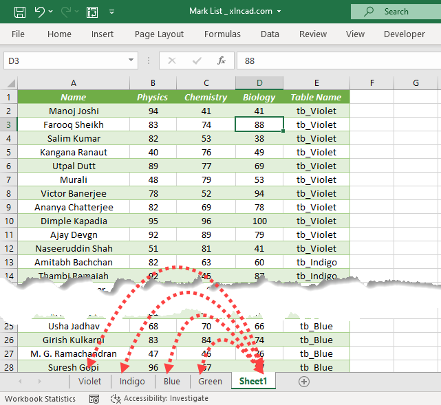
Following is the screenshot of a workbook which contains 4 worksheets called Violet, Indigo, Blue and Green.
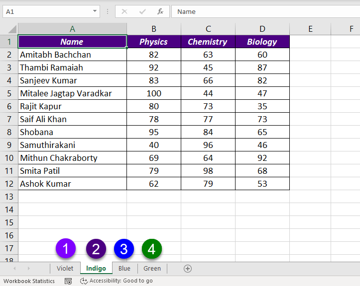
These 4 worksheets contains the marks scored by more than 40 candidates for their Physics, Chemistry and Biology exams. Based on different criteria, these candidates are divided into the 4 groups called Violet, Indigo, Blue and Green.
Now, I want to combine these data into a single worksheet for further analysis. Let’s see how to do that using Power Query.
Step 1:
First step in this method is to convert the data into Excel Tables and name them. If your data is already in Excel Table format, you can skip this method and go to Step 2:
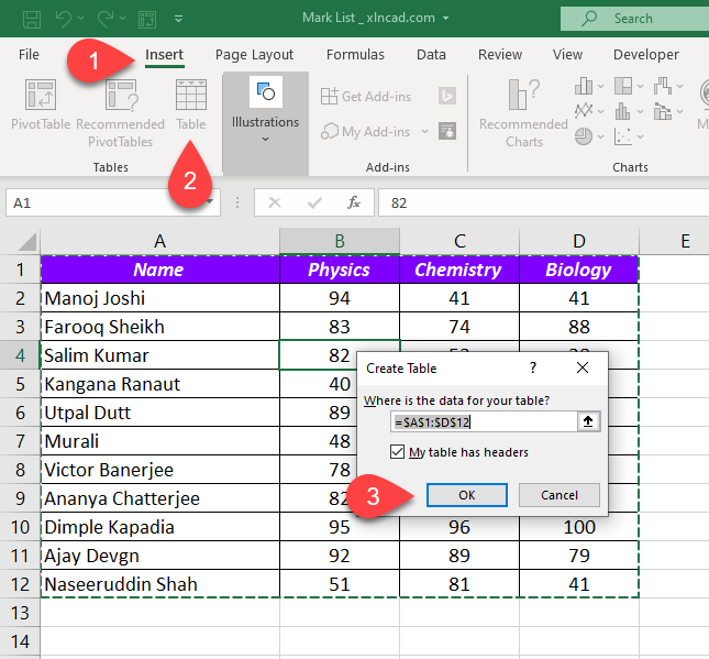
To convert a data range into an Excel Table,
Select a cell in the data range > go to Insert Tab of the Excel ribbon > Click on Table > Create Table dialog will be activated > Click OK
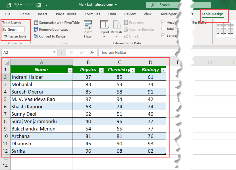
To name an Excel Table,
Select a cell in the Table > go the contextual tab called Table Design > Type in the name into the input box under the label, Table Name. Here, I have used the name Violet for the table, in the worksheet with the same name.
Note: Naming a table is optional, but it becomes easier to refer and handle tables when they are properly named.
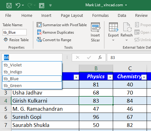
I have created 4 tables and named them as tb_Violet, tb_Indigo, tb_Blue and tb_Green.
The prefix ‘tb_’ was added for specific purpose and will be explained later in this post.
Step 2:
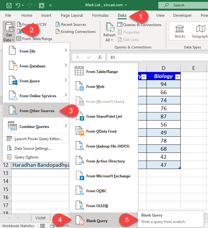
Click on Get Data in the Data tab of Excel Ribbon > From Other Sources > Blank Query > Blank Query
Step 3:
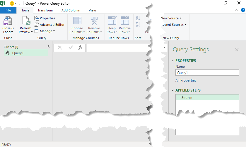
Power Query Editor will be activated with a Blank Query.
Step 4:
To list all those Tables and Named Ranges available in the current workbook, type in the following formula into the formula bar of the Power Query Editor
= Excel.CurrentWorkbook()
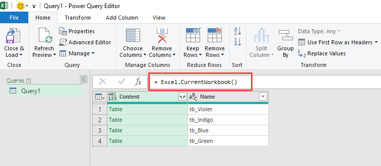
All 4 Tables present in this workbook, i.e. tb_Violet, tb_Indigo, tb_Blue and tb_Green are listed as Tables in the column called Content and their names are listed in the second column called Name
Step 5:
To make sure, this Query will only consider those tables whose names starts the prefix tb_,
Click on the Filter button of the column called Name > Text Filters > Begins With…
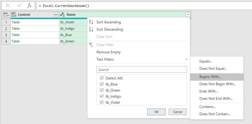
In the dialog for Filter Rows, against the drop down menu begins with, type in tb_ and click OK
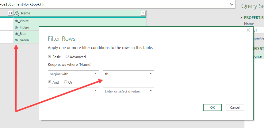
This action will filter only the tables whose name start with the characters ‘tb_’. This is why I have used the prefix tb_ while creating tables.
Step 6:
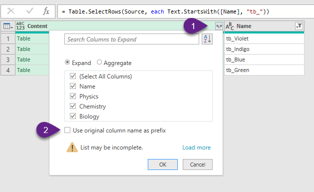
To expand the tables in the column called Content, click on the double headed arrow of the column header > Select the radio button for Expand > UnMark the checkbox against the label ‘Use original column name as prefix’ > Click OK
As you can see below, data from 4 different sheets is consolidated into a single table.
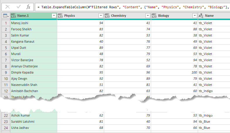
You can change the column headers or remove any of these columns if you want to.
Even if, I don’t want the last column containing table names for analysis, I will rename it as Table Name and keep it to explain the dynamic nature of this query.
Step 7:
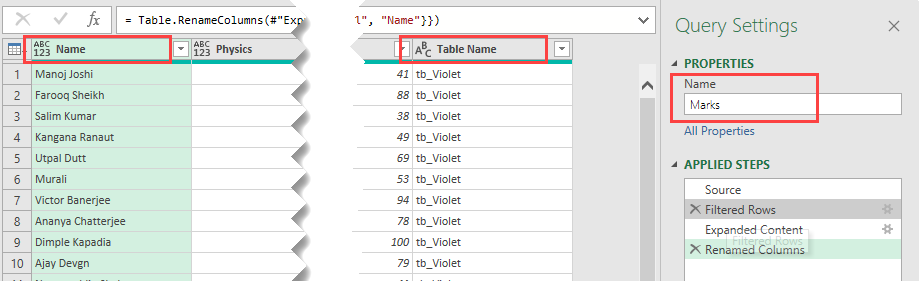
Rename the Query and the Column headers.
I will rename the Query as Marks.
The column ‘Name’ will renamed as Table Name and the column ‘Name.1’ as ‘Name‘.
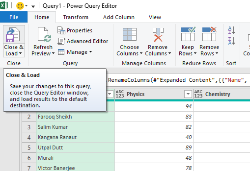
Step 8:
To load this data into an Excel worksheet,
Click on Close & Load in the Home tab of the Power Query Editor.
A new worksheet is created which contains the consolidated data from 4 worksheets present in this workbook.
Like I told you earlier, this query is pretty dynamic and can handle addition of new worksheets.
Here I have added 3 new worksheets Yellow, Orange and Red which contains data in 3 tables tb-Yellow, tb_Orange and tb_Red.
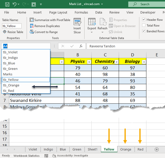
To update the output table for the newly added data, right click on the table and select Refresh. You can also use the Refresh button in the Data tab of the Excel ribbon for the same.
Data from the 3 worksheets Yellow, Orange and Red got appended to the table called Marks.
Similarly, when you delete sheets, containing tables and refresh the Query the output table will update for the same.