In this blog post, I will explain the step by step procedure to Connect Google Sheets with Excel using Power Query.
Once a spreadsheet in Google Sheets is connected with an Excel file, the changes made in the Source (Google Sheet) will be reflected in the Excel file at the expense of a single mouse click.
Following is my Google Sheet containing some sample Sales Data. To connect this sheet with an Excel file, Click on the Share button.
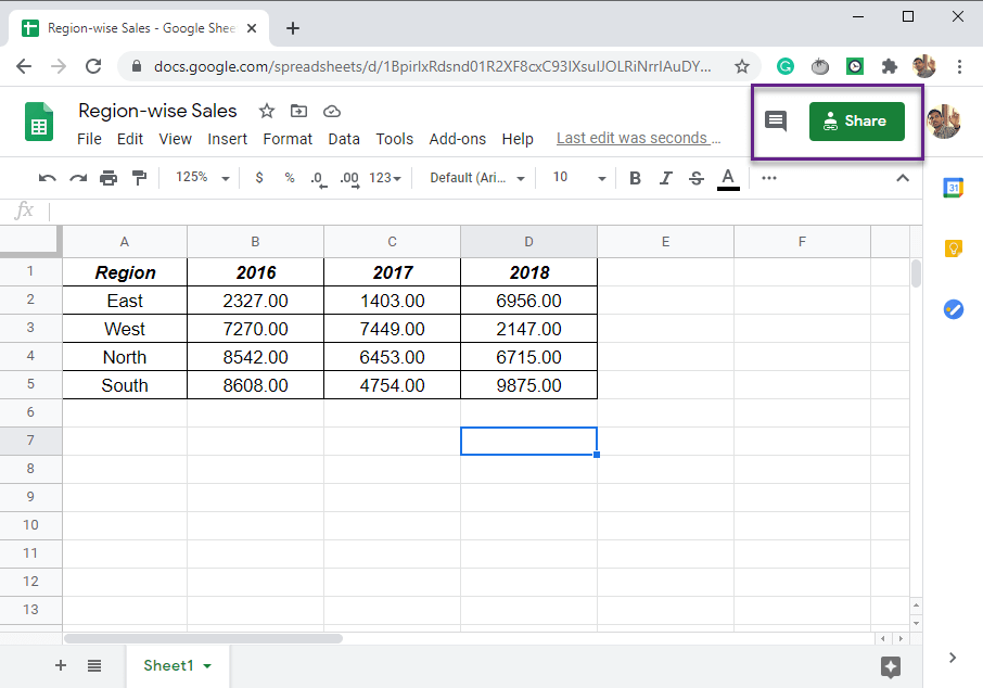
Click on Copy link.
Once the link is copied we will get a message, then click on Done.

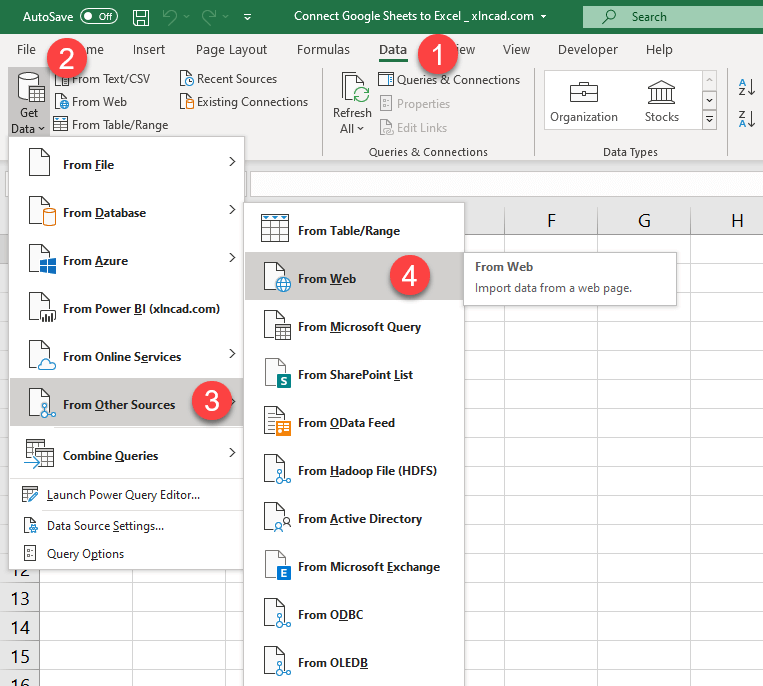
To import data into Excel, Open a new Excel file > go to the Data tab of Excel ribbon > Get Data > From other sources > From Web
Paste the copied link into the dialog called From Web

Next step is the integral part of this method.
replace edit?usp=sharing with export?format=xlsx and click OK

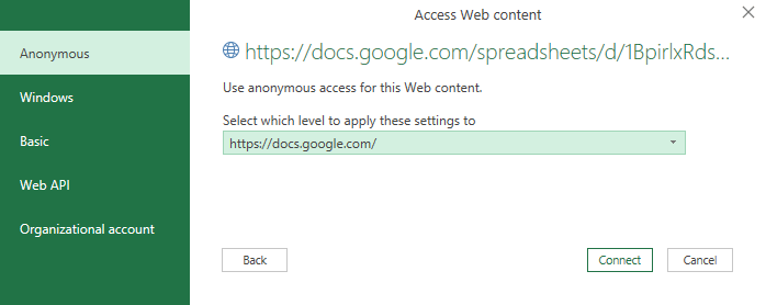
If you are connecting Excel to Google Sheets for the first time you will get a dialog called Access Web Content. Click on Connect.
A new dialog called Navigator is activated and this dialog has the preview of our data in Google Sheets.
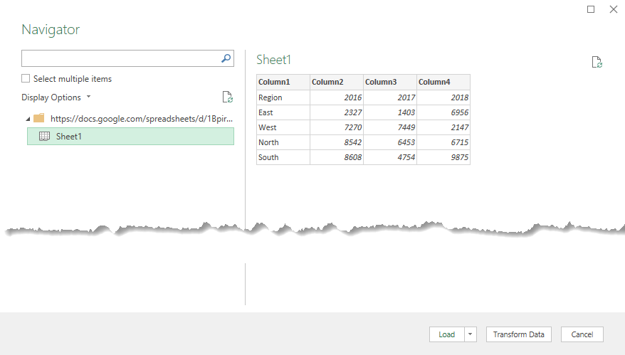
If I click on Load, this data will be loaded into a new Excel Worksheet.
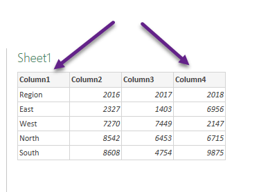
But here we have to make some changes. Excel has detected the column headers as Column1, Column2, etc., To modify the column headers, click on Transform Data.
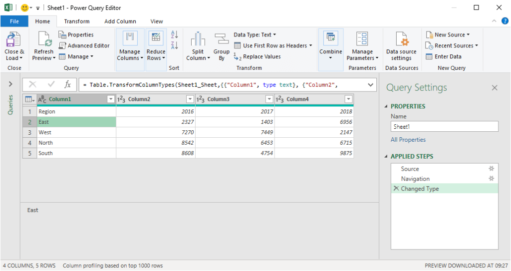
Selected data is loaded into the Power Query Editor of Excel.
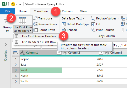
Right now the column headers of the data i.e. Region, 2016, 2017, and 2018 are in the first row. To promote this first Row to column headers, go to Transform tab of Power Query Editor > Click on Use First Row as Headers
The first row is promoted as column headers.
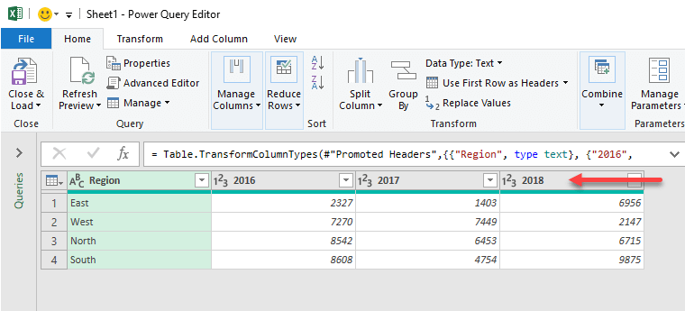
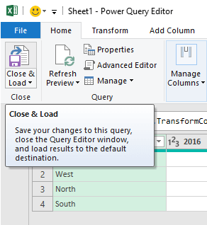
To load this data into the Excel worksheet, click on Close & Load in the Home tab
Data in the Google Sheets is loaded into the Excel worksheet.
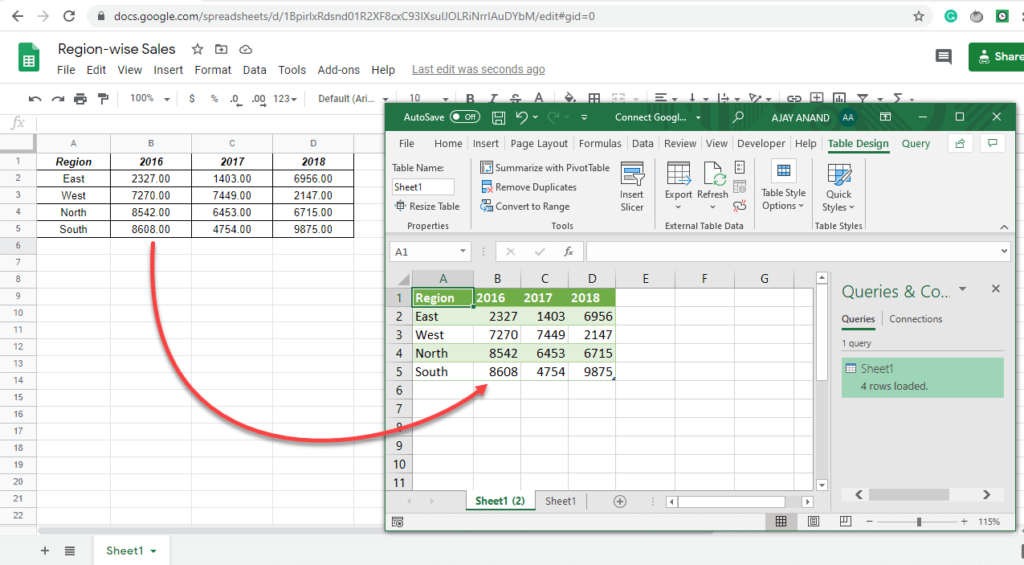
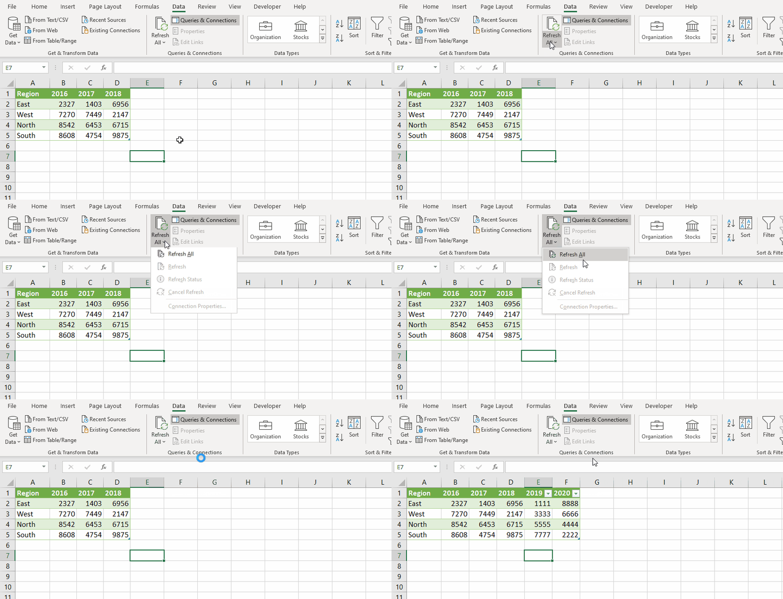
Now, when I make a change in the Google sheets, I can import that change into the Excel worksheet by clicking on the Refresh button in the Data tab of the Excel ribbon.
Here, I have added 2 new columns to the Google Sheet.
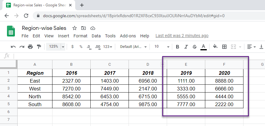
To update the Excel worksheet for this change, click on the Refresh All button in the Data tab.
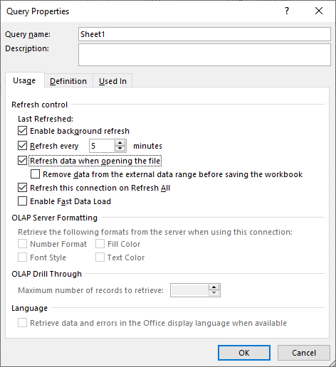
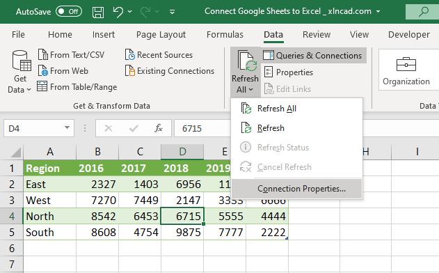
For this Excel file to update at periodic intervals, select the Table containing data > click on the down arrow under Refresh All > Connection Properties
Mark the checkboxes for the following and click OK
- Refresh every n minutes (Specify the number of minutes)
- Refresh data when opening the file
