Following are 10 different methods to create a Number Series (1, 2, 3,… 49, 50) in Excel.
Table of Contents
Excel Fill Handle to create Serial Numbers
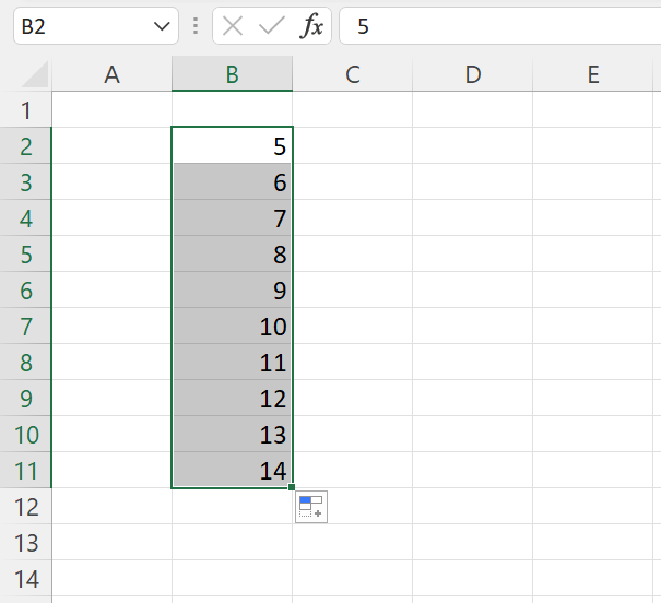
To create a number series like 5, 6, 7,… up to the number14,
type 5 into a cell > 6 into the cell just below it > select these two cells > using the Excel Fill Handle drag down
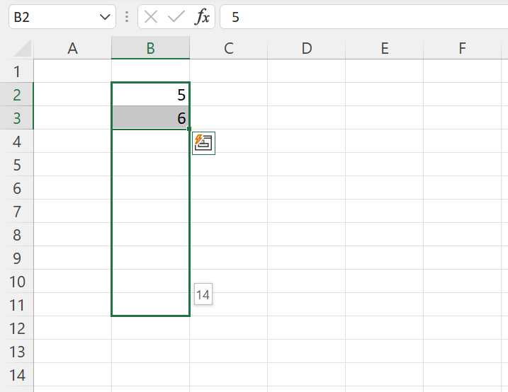
release the mouse button after 9 cells and the cells up to that point will be filled with numbers from 5 to 14.
Less known trick with Excel Fill handle
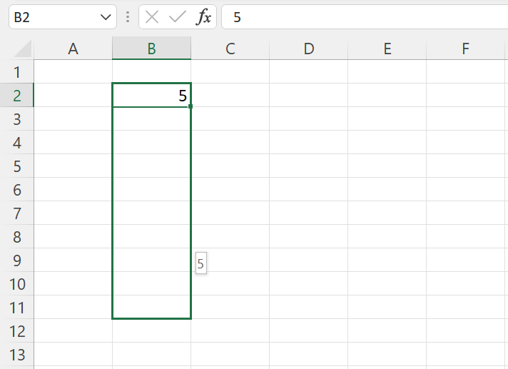
Type in 5 into a cell. Holding the Ctrl key, drag the Excel Fill Handle down.
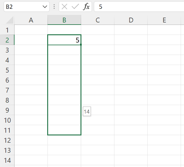
release the mouse button after 9 cells and the cells up to that point will be filled with numbers from 5 to 14.
Auto Fill for creating Serial Numbers
Type in the first number of the series into a cell. Here the first number of the required series is 5.
Click on the Excel Fill Handle and drag down.
When you release the mouse button, the cells up to that point will be filled with the same number.
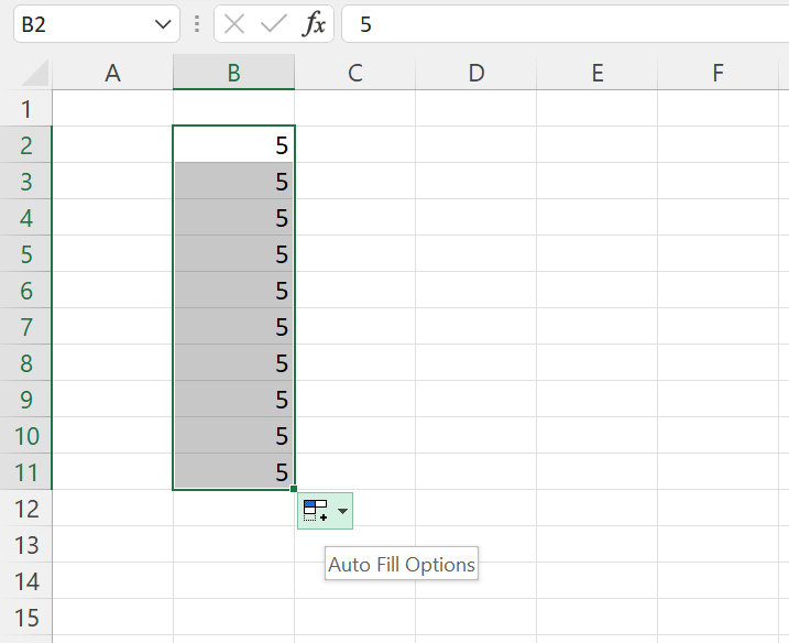
Click on the split button for Auto Fill Options
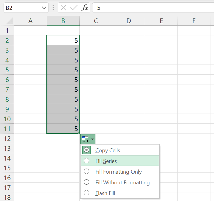
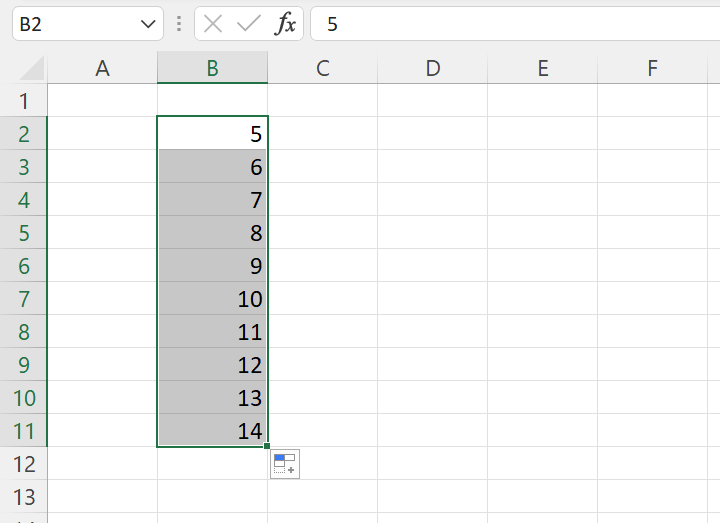
Select Fill Series and the highlighted cells will be filled with the corresponding Number Series.
Adding one to the previous value
Type the starting number of the required series into a cell. In the adjacent cell down, create a formula which will add 1 to the above value.
Here I have the number 5 in the cell B2 and the formula in the cell below will be,
=B2+1
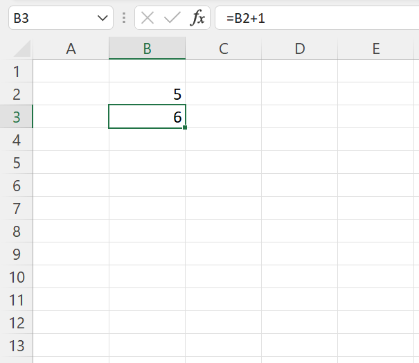
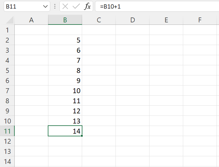
Copy the formula downwards up to the cell B11 and we will have the number series from 5 to 14.
Fill Series
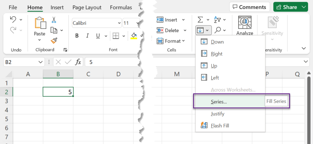
Type in the number 5 into a cell.
In the Home tab > Fill > Series…
In the dialog called Series,
click on the radio button for Columns, type in 1 in the input box for Step value: and 14 in the input box for Stop value:
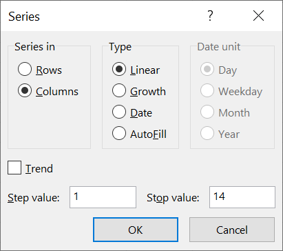
Click on OK and we will have a Number Series from 5 to 14.
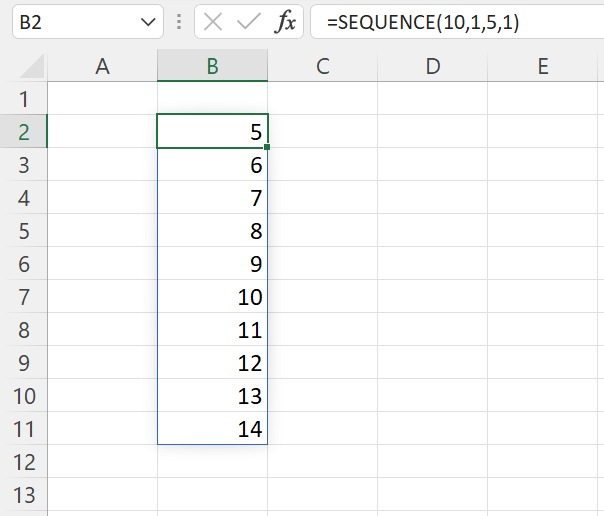
SEQUENCE Function
The SEQUENCE function in Excel can be used to create a Single or Multi dimensional array of numbers in the required interval.
Following is the formula to generate a Number Series, starting from 5 to 14.
=SEQUENCE(10,1,5,1)
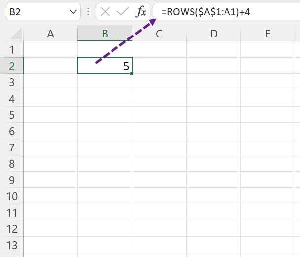
ROWS Function
The ROWS function in Excel returns the number of rows in the Range Reference supplied into it.
The following formula is used to create the number 5 in the cell B2
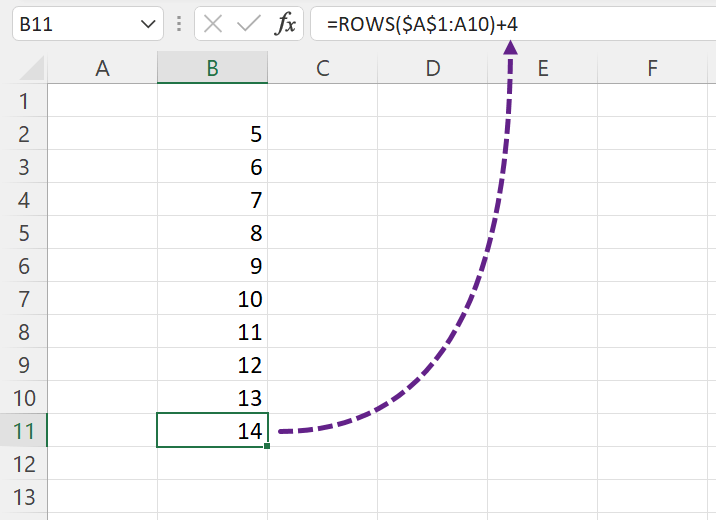
=ROWS($A$1:A1)+4
Copy the above formula up to the cell B11 and we will have a number series from 5 to 14.
ROW Function
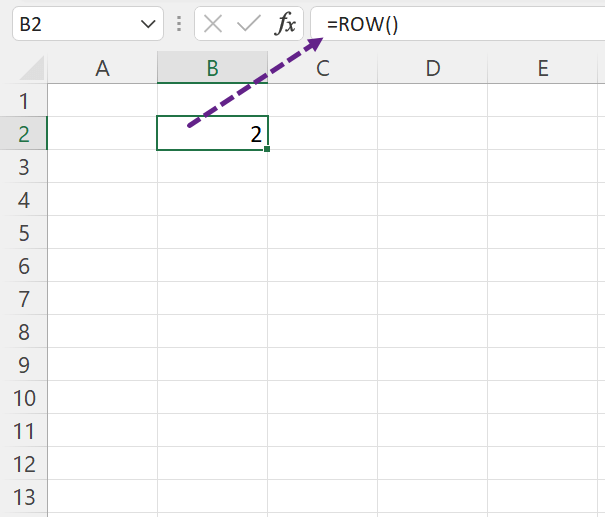
The ROW function in Excel will return the Row Index of the cell reference used in it. If nothing is specified inside ROW functon, ROW function will return the row index of the cell in which the function is used.
When ROW function is used in the cell B2, it will return the value 2.
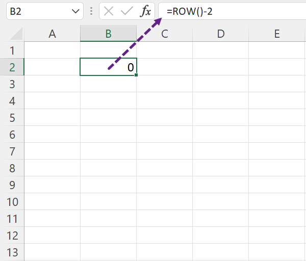
Subtract 2 from this formula to get 0 as result.
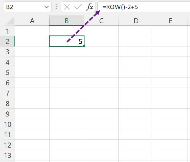
Add 5 to the formula to fix 5 as the starting number in the series.
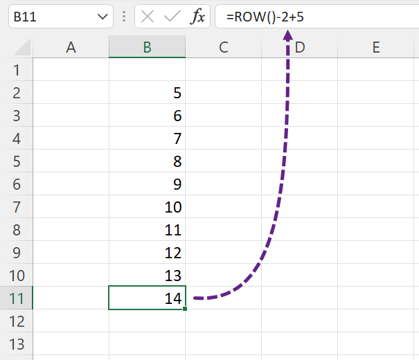
Copy this formula up to the cell B11 and we will have the numbers from 5 to 14.
Power Query
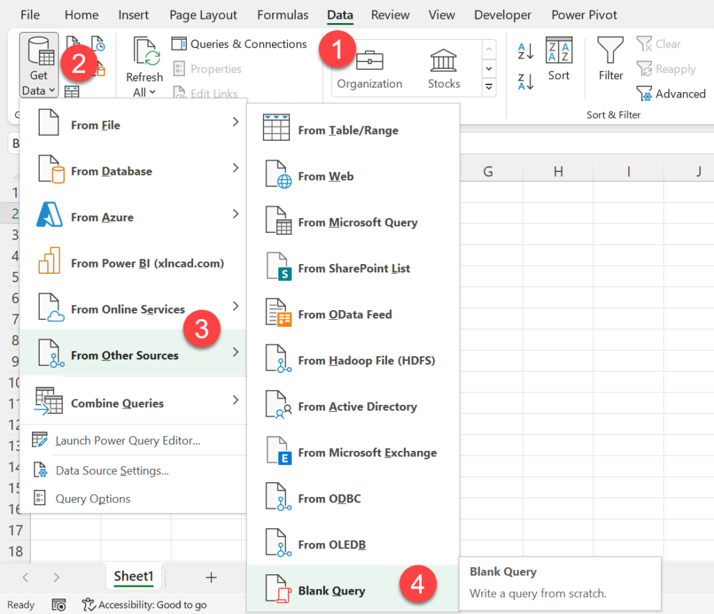
To create a Number Series using Power Query in Excel,
In the Data tab of the Excel Ribbon > Get Data > From Other Sources > Blank Query
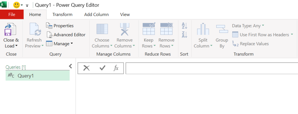
The Power Query Editor of Excel is activated.
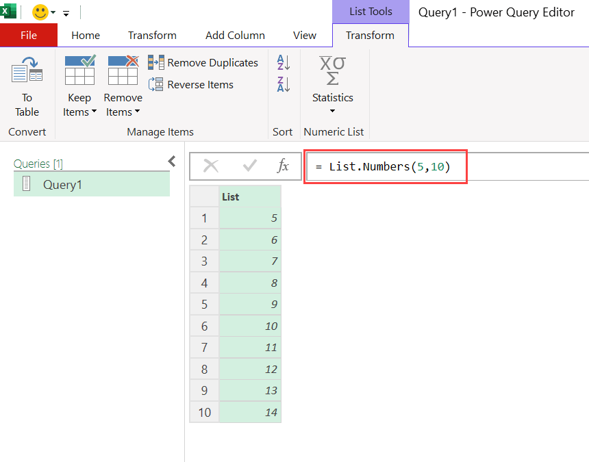
In the formula bar of the Power Query Editor, type in the following formula and press Enter.
= List.Numbers(5,10)
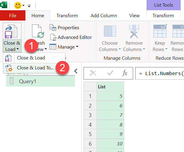
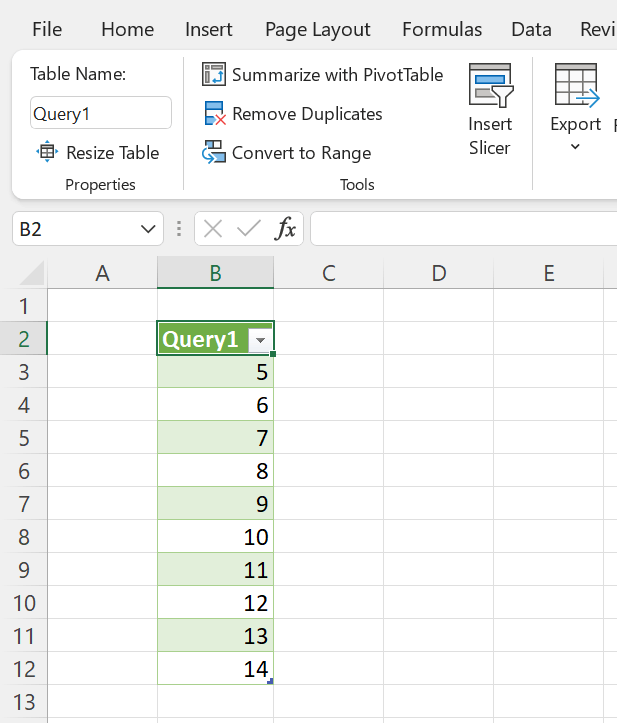
To load these serial numbers into an Excel Worksheet,
in the Home tab of the Power Query Editor > click on the split button for Close & Load > Close & Load To…
Using the Import Data dialog, specify the location where you want to place the table containing numbers
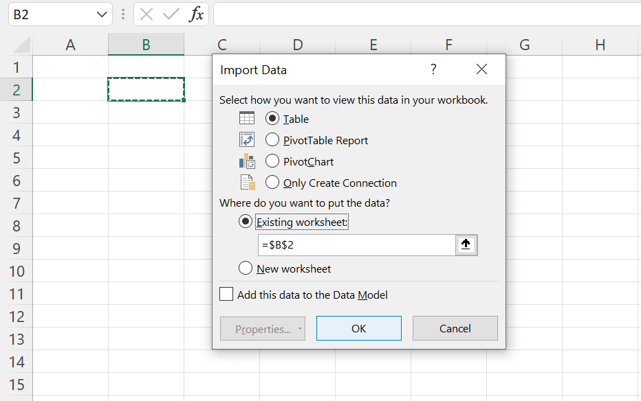
The table containing numbers from 5 to 14 is loaded into the Excel Worksheet.
Macro to create Number Series
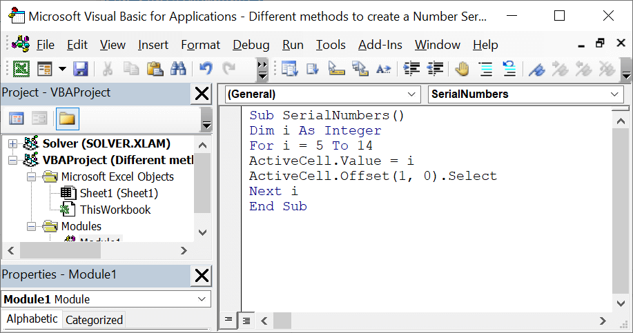
The following macro when executed will generate a series of numbers from 5 to 14.
Sub SerialNumbers()
Dim i As Integer
For i = 5 To 14
ActiveCell.Value = i
ActiveCell.Offset(1, 0).Select
Next i
End Sub
Copy and paste the above code into the VBA Editor of Excel
Go to the Developer tab in the Excel ribbon > Macros > execute the Macro called SerialNumbers to generate a series of numbers from 5 to 14.