In Excel, we have the VLOOKUP function to perform Lookup in Vertical direction (Rows) and the HLOOKUP function to Lookup in Horizontal direction (Columns).
But for 2 Way Lookup? i.e. to perform Lookup in both columns and rows?
No. Excel doesn’t have a dedicated function for this purpose. We should create the formula for 2 Way Lookup using the available Excel functions.
This tutorial is about 3 different formulas which can be used to perform Two Way Lookup in Excel.
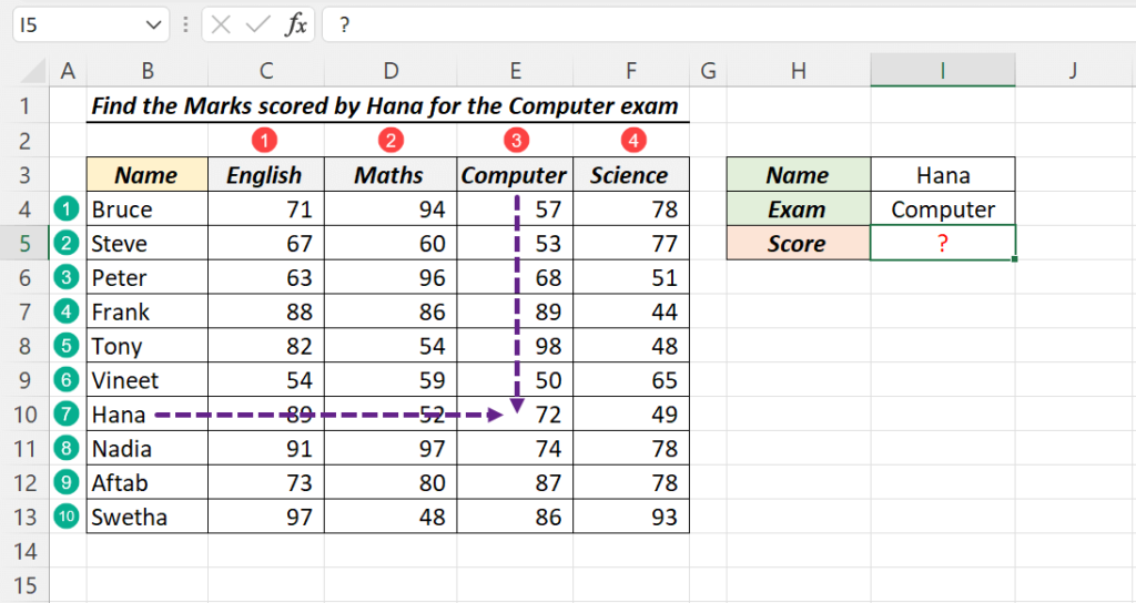
Following is the data set used for this purpose and our aim to find the Marks scored by ‘Hana’ for her ‘Computer’ exam.
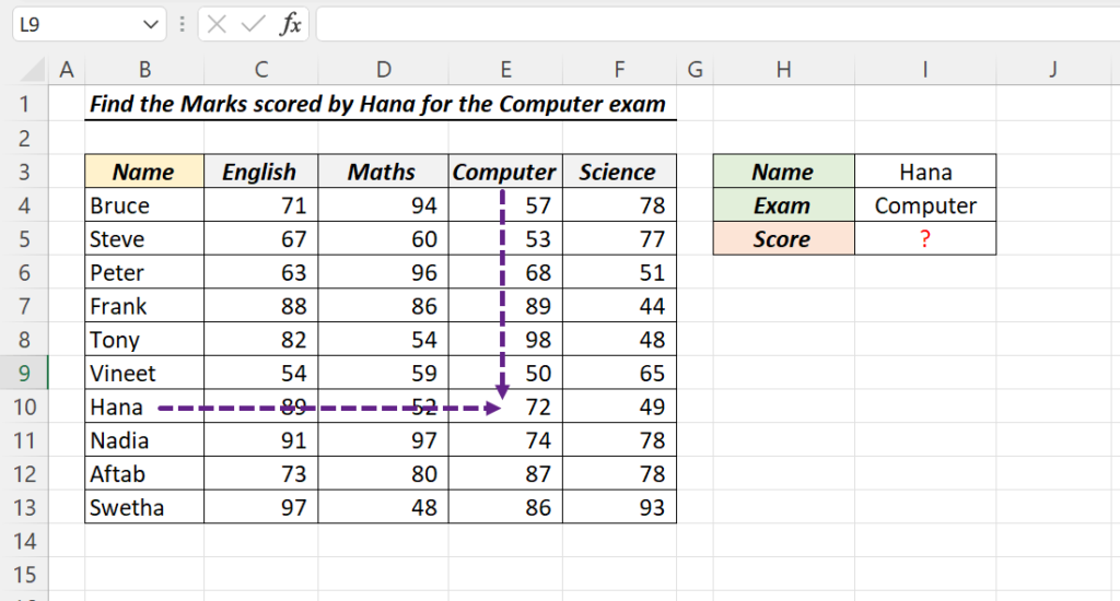
Table of Contents
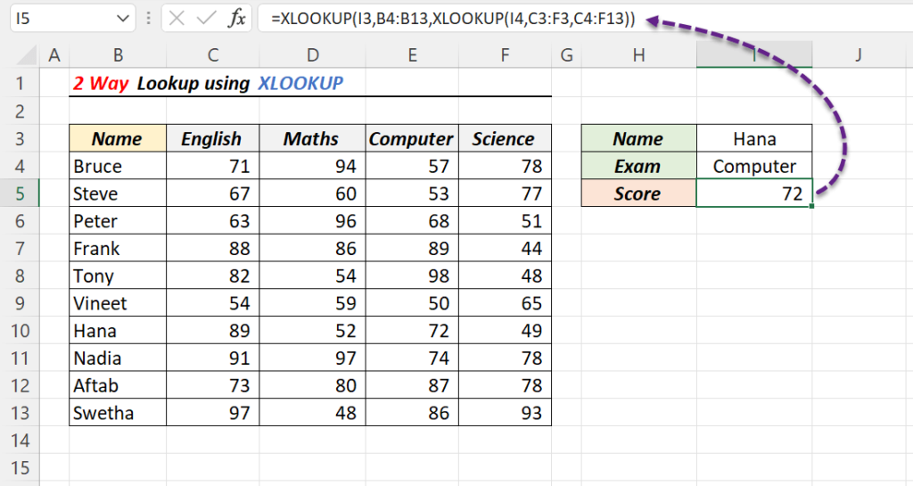
2 Way Lookup using XLOOKUP function
Nesting the XLOOKUP function inside another is one of the fastest ways to perform 2 Way Lookup in Excel.
The following formula will return the marks scored by Hana for her Computer exam.
=XLOOKUP(I3,B4:B13,XLOOKUP(I4,C3:F3,C4:F13))
In the above formula, the second/inner XLOOKUP function will search for the value ‘Computer’ in the cells containing name of Exams (C3:F3) and will return the array of Marks in the corresponding column (57, 53, 68, 89, 98, 50, 72, 74, 87, 86). This array will become the third argument of the first/outer XLOOKUP function.
=XLOOKUP(I4,C3:F3,C4:F13)

={57;53;68;89;98;50;72;74;87;86}
The first/outer XLOOKUP function will search for ‘Hana’ in the cells containing name of the Candidates (B4:B13) and when found will return the corresponding mark from the array generated using the second/inner XLOOKUP function.
=XLOOKUP(I3,B4:B13,XLOOKUP(I4,C3:F3,C4:F13))

=XLOOKUP("Hana",{"Bruce";"Steve";"Peter";"Frank";"Tony";"Vineet";"Hana";"Nadia";"Aftab";"Swetha"},{57;53;68;89;98;50;72;74;87;86})

=72
2 Way Lookup using VLOOKUP
The VLOOKUP function is designed to search for the Lookup value in the first column of a table and return the corresponding value from the specified column of that table. Normally this column number will be hard coded inside VLOOKUP function. But, using the MATCH function we can make this column number dynamic and force the VLOOKUP function to perform a 2 Way Lookup.
The following formula will return the marks scored by Hana for her Computer exam.
=VLOOKUP(I3,B4:F13,MATCH(I4,B3:F3,0),FALSE)

In the above formula, MATCH function will search for the value ‘Computer’ in the cells from B3:F3 and will return the value 4.
=MATCH(I4,B3:F3,0)

=4
The value 4, returned by MATCH function will become the 3rd argument of VLOOKUP function and will return the score from 4th column of the table.
=VLOOKUP(I3,B4:F13,MATCH(I4,B3:F3,0),FALSE)

=VLOOKUP("Hana",{"Bruce",71,94,57,78;"Steve",67,60,53,77;"Peter",63,96,68,51;"Frank",88,86,89,44;"Tony",82,54,98,48;"Vineet",54,59,50,65;"Hana",89,52,72,49;"Nadia",91,97,74,78;"Aftab",73,80,87,78;"Swetha",97,48,86,93},4,FALSE)

=72
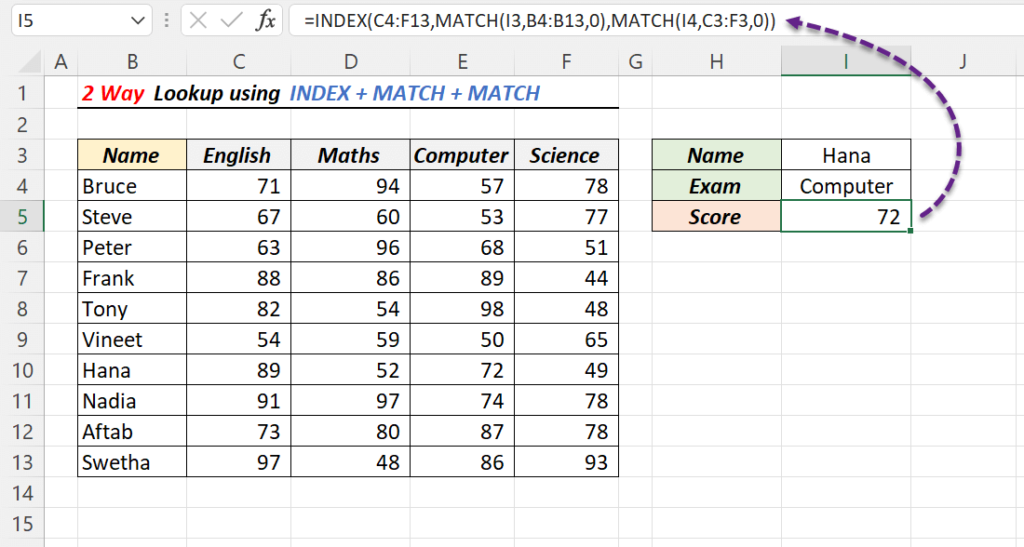
2 Way Lookup using INDEX and MATCH functions
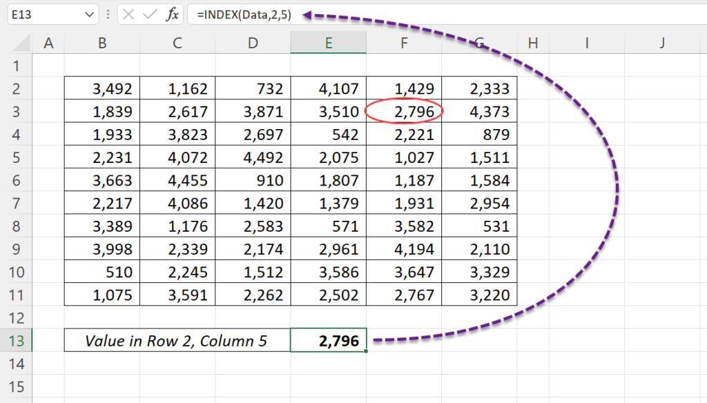
The INDEX function in Excel can be used extract the value present in the specified location of a Table or an Array. The location is defined using the Row and Column number.
The formula =INDEX(Data, 2, 5) will return the value present in the 2nd row of the 5th column of the table called Data.
To find the row and column numbers corresponding to the lookup values, we will use the MATCH function.
To get the Row number corresponding to the Candidate ‘Hana’,
=MATCH(I3,B4:B13,0)

=7
To get the Column number corresponding to the Exam ‘Computer’,
=MATCH(I4,C3:F3,0)

=3
C4:F13 is the data range containing Marks.
Combining all these, the formula will become
=INDEX(C4:F13,MATCH(I3,B4:B13,0),MATCH(I4,C3:F3,0))

=72