This article is about 3 different methods to Reverse a List in Excel.
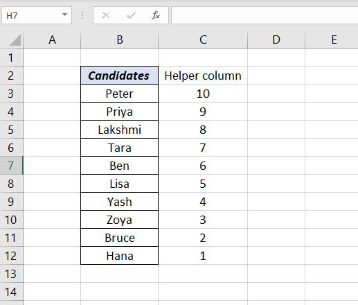
Following is a list of candidates applied for a job. Let’s see the different methods to reverse this list for scheduling the interview.
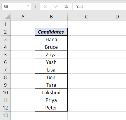
Table of Contents
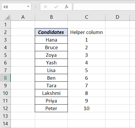
1. Reverse the list using a Helper column
Create a helper column with sequential numbers (for example 1,2,3,..) adjacent to the column containing the list.
Select any of the cells in the helper column > go to the Data tab of Excel ribbon > Click on Sort Largest to Smallest
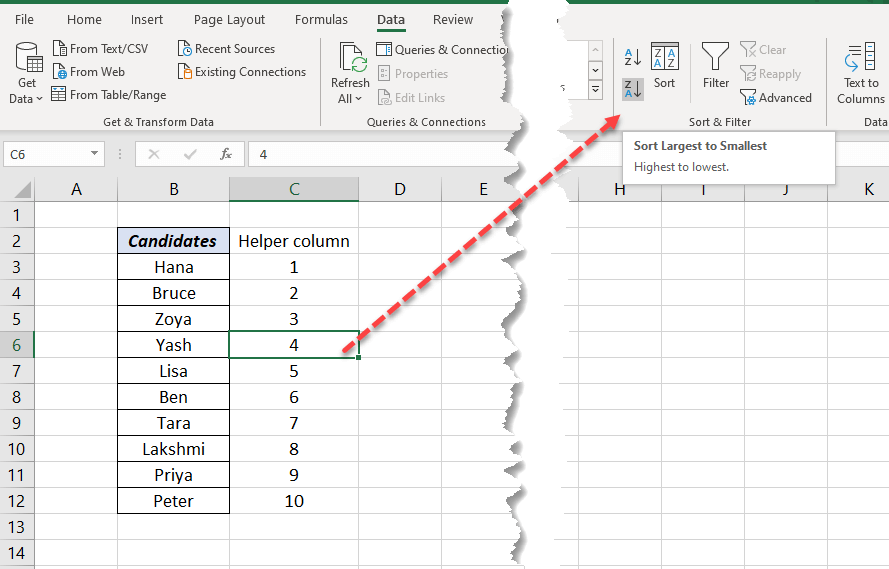
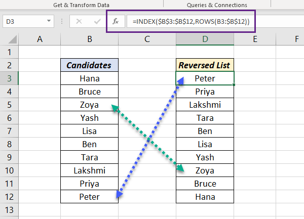
The list in column B as well as C has been reversed. ‘Peter’, who was at the bottom of the list came to the top.
2. Reverse the list using a Formula
By combining INDEX function with ROWS function we can reverse the order of a list in Excel.
To reverse the list of values in the cells B3:B12, type in the following formula into a cell and copy the formula into the downward cells. (Here the length of the list is 10, so copy the formula into 9 cells below.)
=INDEX($B$3:$B$12,ROWS(B3:$B$12))
Explanation
The data range containing the list i.e. B3:B12 becomes the first argument array of the INDEX function.
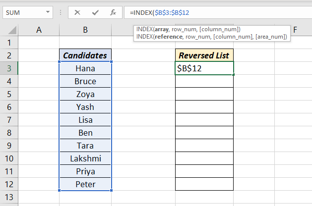
To return the last item from this array, ROWS function is used.
ROWS(B3:$B$12) will evaluate to 10 and will return ‘Peter’ which is the 10th Name in the list.
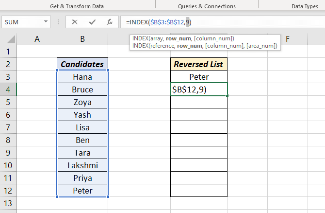
When copied down to the adjacent below, ROWS(B3:$B$12) will become ROWS(B4:$B$12). This expression will be evaluated to 9 and will return ‘Priya’ which is the 9th Name in the list.
Reverse a list using Power Query
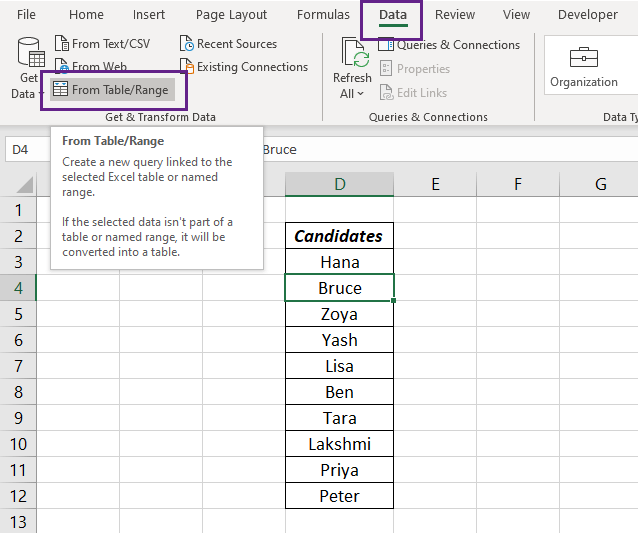
Power Query in Excel also can be used to reverse a List of values or an entire Table.
To reverse the list of candidates, select the cells containing data > Click on From Table/Range in the Data tab of Excel ribbon.
Create Table dialog will be activated.
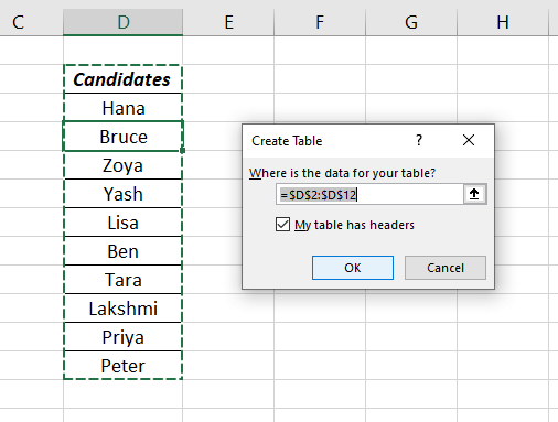
Click OK and the data will be loaded into the Power Query Editor.
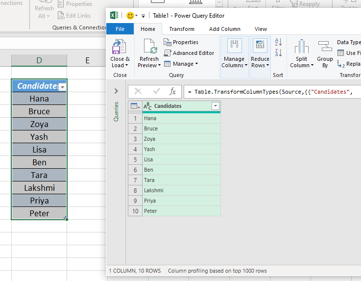
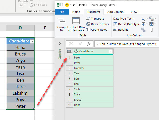
Go to the Transform tab of the Power Query Editor and click on Reverse Rows.
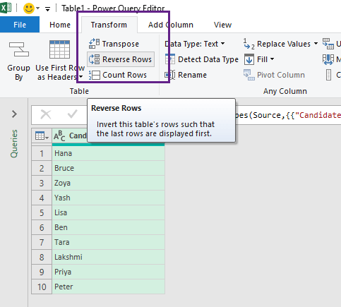
See the list has been reversed.
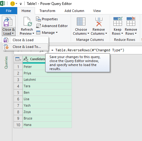
To load this data into an Excel sheet, in the Home tab of the Power Query Editor > Close & Load > Close & Load To…
In the dialog called Import Data, select the radio button for the Existing worksheet > select the cell where you want to load the data. In this case, I have selected the cell G2.
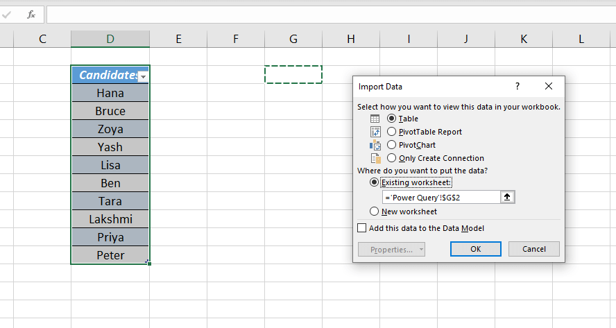
Click OK and the reversed list will be loaded into the cell G2.
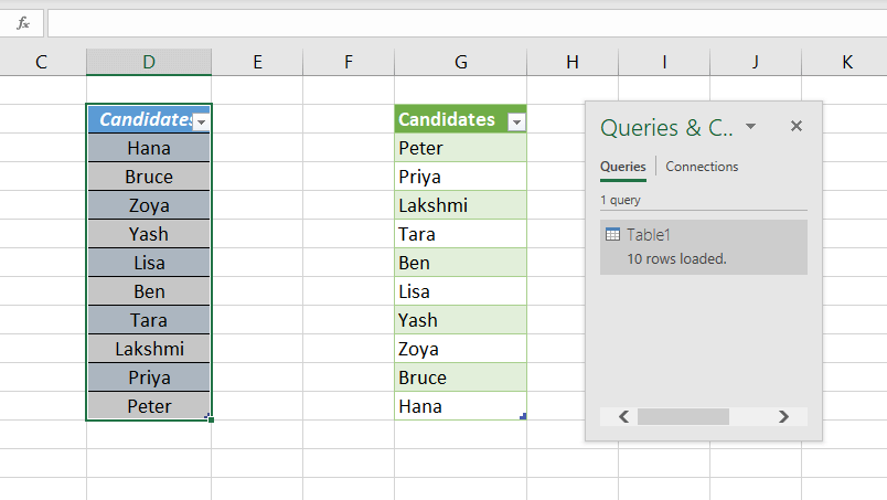
This is the most dynamic one among all 3 methods explained here. If you plan to add more items to the list, you can update the output table with a single click on the Refresh button in the Data tab of the Excel ribbon.