Table of Contents
About
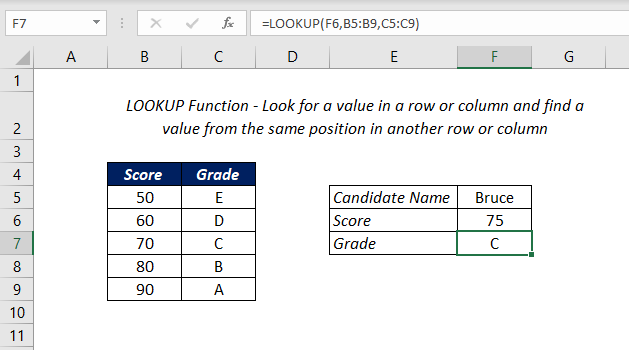
The Excel LOOKUP function is a LOOKUP & REFERENCE function that is used to search a value in a single row/column and return the corresponding value from the second row/column.
Function Type
Lookup and reference
Vector Form of Lookup Function
LOOKUP function has two forms, Vector and Array. We will see the Vector form first.
Use the vector form of LOOKUP function when you want to specify the range that contains the values that you want to match.
Purpose
Look for a value in a row/column and return the corresponding value from the second row/column.
Return value
A value in the result vector.
Syntax
=LOOKUP(lookup_value, lookup_vector, [result_vector])
Arguments
lookup_value – The value LOOKUP searches for in the first vector. This can be a number, text, a logical value, or a name or reference that refers to a value
lookup_vector – that one-row, or one-column range to search
result_vector – that one-row, or one-column range containing results. this should be of the same size that of lookup_vector
Examples
Grade from the Score of a Candidate
In this example, we will see how to use the LOOKUP function to return the Grade after analyzing the score of a candidate.
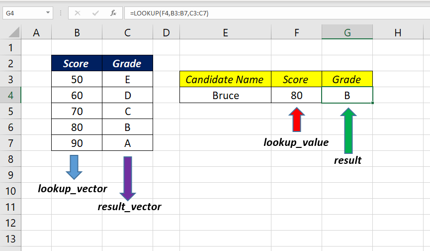
The following formula will return the Grade of the score 80 in the cell F4 after comparing it with the Grade and Score Matrix in the range B3:C7.
=LOOKUP(F4,B3:B7,C3:C7)
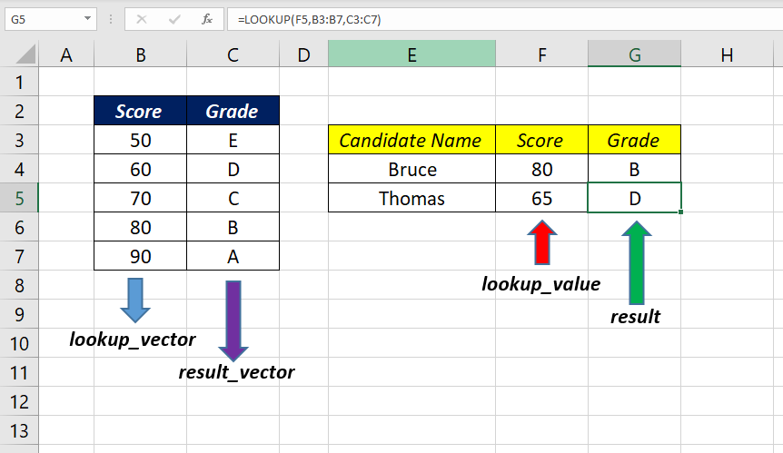
If the LOOKUP function can’t find an exact match, the function will return the value corresponding to the next smallest value.
In this case, if we search for the Grade of the score 65, LOOKUP function will return the value D
=LOOKUP(F5,B3:B7,C3:C7)
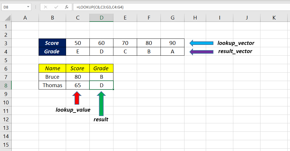
LOOKUP function can also perform lookups in the horizontal direction.
In the following example, I have aligned the same data (Grade/Score Matrix) in columns (C3:G4) and used LOOKUP function to find the Grade corresponding to the candidate score in the cells C7 and C8
=LOOKUP(C8,C3:G3,C4:G4)
Array Form of Lookup Function
The array form of LOOKUP function looks in the first row or column of an array for the specified value and returns a value from the same position in the last row or column of the array. This form of LOOKUP function is used when the value that needs to be matched is in the first row or column of the array.
Purpose
Look for a value in a row/column and return the corresponding value from the second row/column.
Return value
A value from the last column or row of the array.
Syntax
=LOOKUP(lookup_value, array)
Arguments
lookup_value – The value LOOKUP searches for in the first vector. This can be a number, text, a logical value, or a name or reference that refers to a value
array – A range of cells that contains text, numbers, or logical values that you want to compare with lookup_value
Example
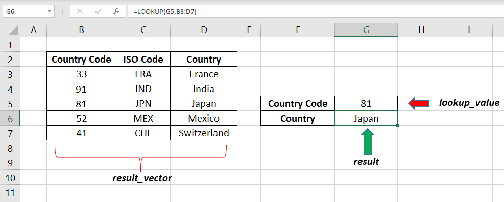
Perform a lookup for the Country name using Country code
In this example, LOOKUP function is used to return the country Name from a table containing Country Code (B3:B7), ISO Code (C3:C7) and Country Name (D3:D7)
The following formula will look for the Country Code 81 (lookup value in the cell G7) in the range of cells from B3:D7 (array) and will return the corresponding country name, Japan.
=LOOKUP(G5,B3:D7)
Notes
LOOKUP function assumes that lookup_vector is sorted in ascending order
result_vector must be the same size as lookup_vector
When lookup-value can’t be found, the LOOKUP function will match the next smallest value
When lookup_value is greater than the greatest value in lookup_vector, LOOKUP matches the last value
When lookup_value is less than the smallest value in lookup_vector, LOOKUP returns #N/A error
LOOKUP function is not case-sensitive
Excel Functions in Alphabetical Order (Complete list)
Complete List of Excel Functions (Category wise)