I this blog post, I will explain the Fill Up and Fill Down Transformation steps in Power Query of Excel with a simple example.
Following is the collection report of Infinity Saga which comprises of 23 Marvel movies that were released in 3 Phases.

I want to create two reports from this data.
1. Phase-wise Revenue
2. Year-wise Revenue
But the problem here is Pivot Tables are not friendly to the data with blank cells in it. So, before creating Pivot Table reports, I should fill the holes of this data with values in the adjacent cell above and below.

Let’s see how to use Fill Up and Fill Down options in Power Query to fill the blank cells in the above data set.
To load the data into the Power Query Editor,
Select a cell in the data range > Data tab > From Table/Range > Click OK in the Create Table dialog
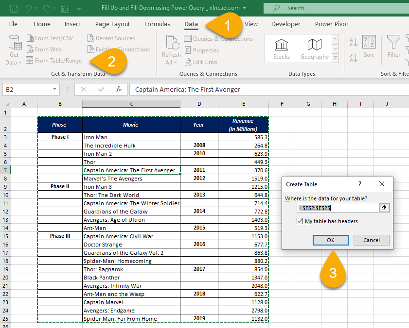
Selected data is loaded into the Power Query Editor
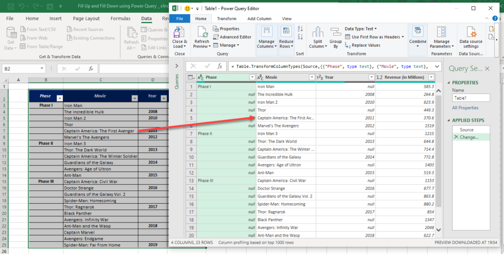
To fill down the values in the first column called Phase, i.e the value Phase I in Row number 1 into the next 5 cells, Phase II in Row number 7 into the next 5 cells and Phase III in Row number 13 into the next 10 cells,
Right-Click on the column header of the column called Phase > Fill > Down
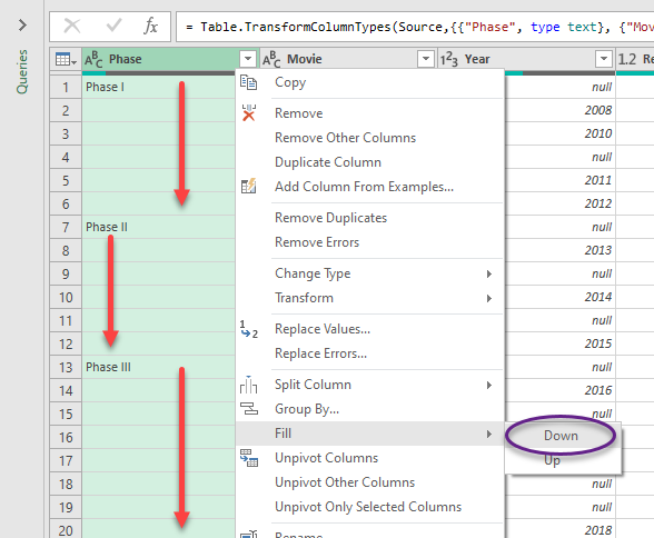
Blank cells in the first column are all filled.

Now, the column called Year. The value in the second row of this column is 2008. This value should be copied into the cell above. In the same manner, all blank cells in this column should be filled with the values in the cell below.
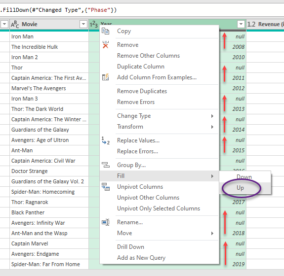
Blank cells in the third column called Year are all filled.

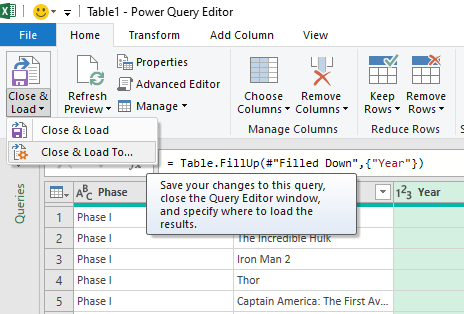
To load this data into the worksheet, Click on Close & Load in the Home Tab > Close & Load to
Select Existing worksheet > Select the cell where you want to place the data (Here, I have selected the cell G2) > Click OK
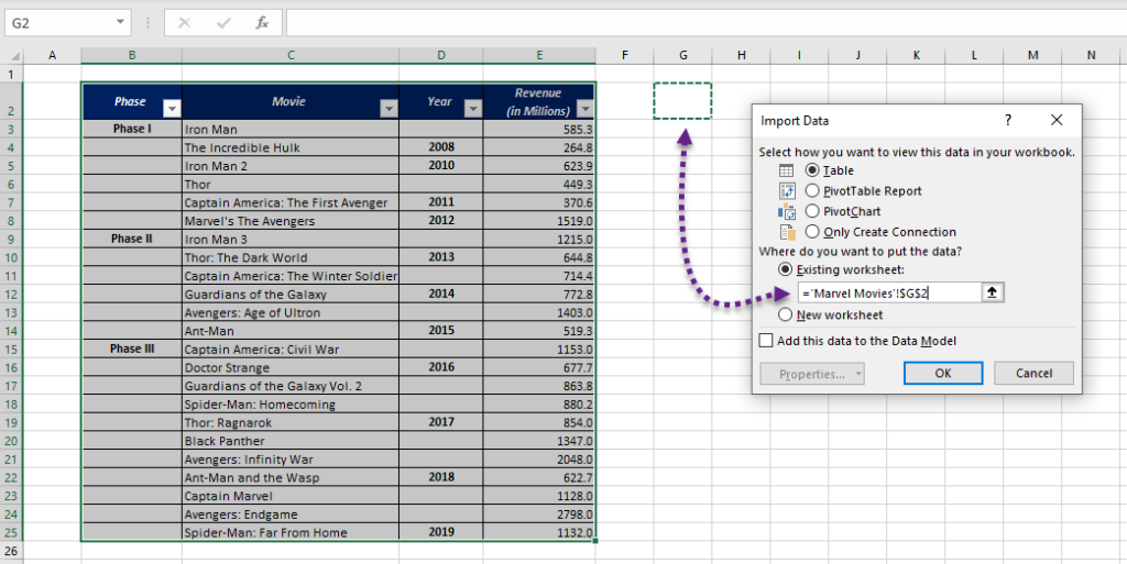
Now, that I have filled the holes in the data set and I can create Pivot Table Reports out of this data

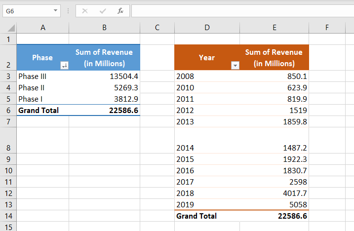
Following is the Pivot Table Reports for Phase-wise and Year-wise revenue, created from the above data.
