I have used at least 7 methods to AutoNumber rows in Excel. But if you ask me, which one is the Easiest and Dynamic method, the answer is… The method using Power Query!
Using Power Query we can add an Index column to data sets and also create Serial Numbers of our choice. Let’s see how to AutoNumber Rows in Excel using Power Query.
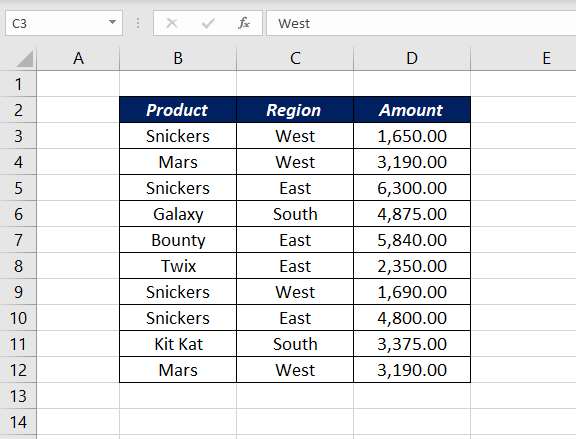
Following is the data set in which I want to add a column containing Serial Numbers
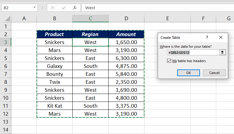
To load this data into the Power Query Editor,
Select a cell in the data set > go to the Data tab > click on From Table/Range > Click OK in the Create Table Dialog
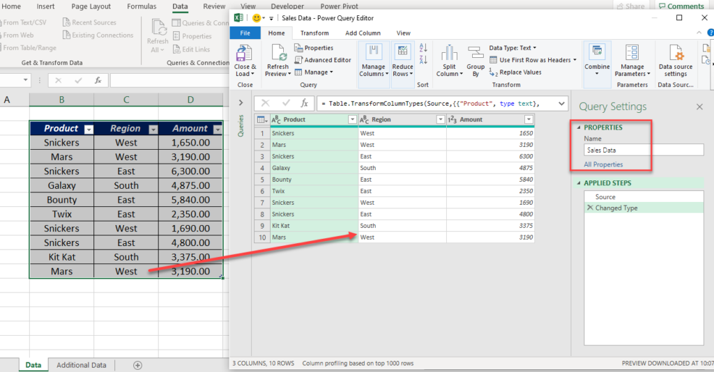
Selected data is loaded into the Power Query Editor.
I have renamed this query as Sales Data [Naming the query is optional, but it is a good practice to name the query as it helps you to handle the queries more efficiently, especially when there 10 or more queries]
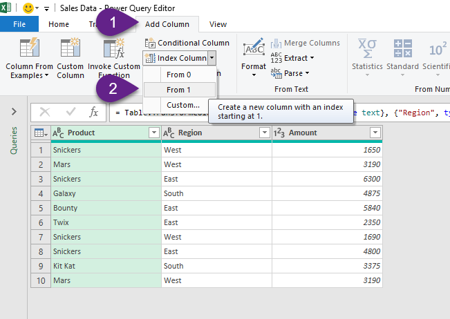
To add an Index column to this data, i.e. a column containing serial numbers, go to the Add Column tab > Click on the small down arrow with Index Column > Select From 1 if you want the numbering to start from One. You can also go for From 0 if you want the first serial number to be Zero.
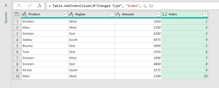
I have selected the option From 1 and a new column called Index is created, which contains a series of numbers starting from 1 up to 10.
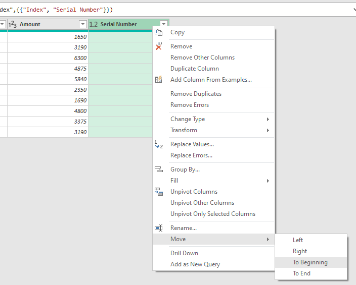
If you want to change the column header, double click on the Column header and type in the column name. Here, I have renamed the column containing serial numbers as Serial Number.
To reposition the column, right-click on the column header > Move > To Beginning
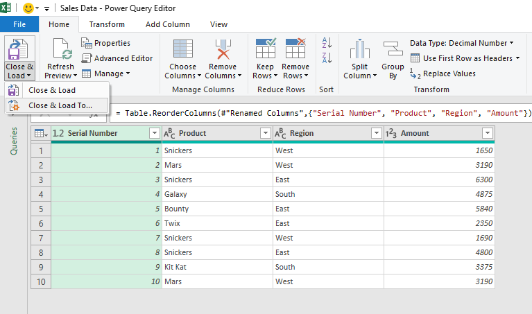
To load this data into the Excel worksheet > Home tab > Close & Load > Close & Load to
In the Import Data dialog, select Existing worksheet > select the cell where you want to place the transformed table (Here, I have selected the cell F2)
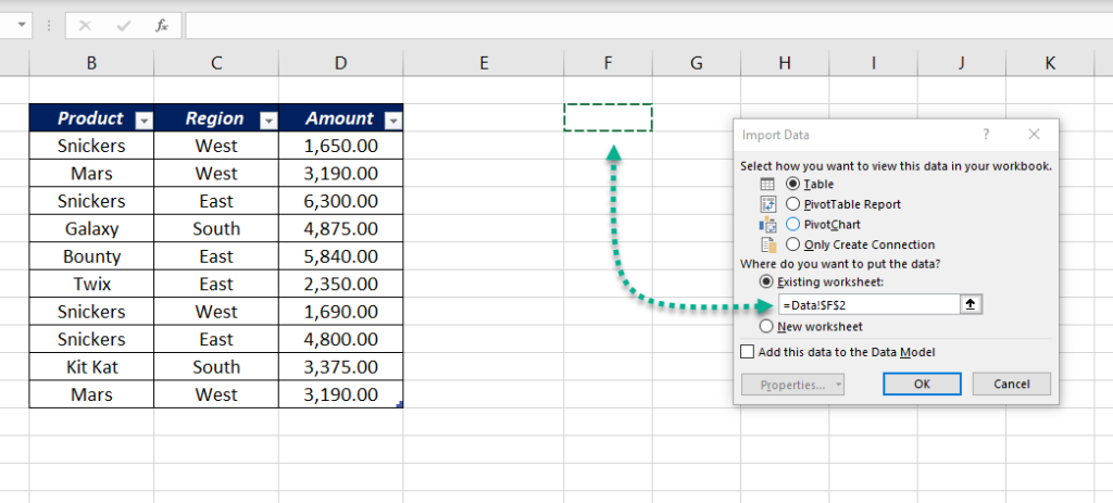
Table on right of the following picture is the transformed data set containing an additional column for Serial Numbers
Whenever you make a change in the source table, right-click on the output table and select Refresh to update it.
Customize Serial Number using Power Query
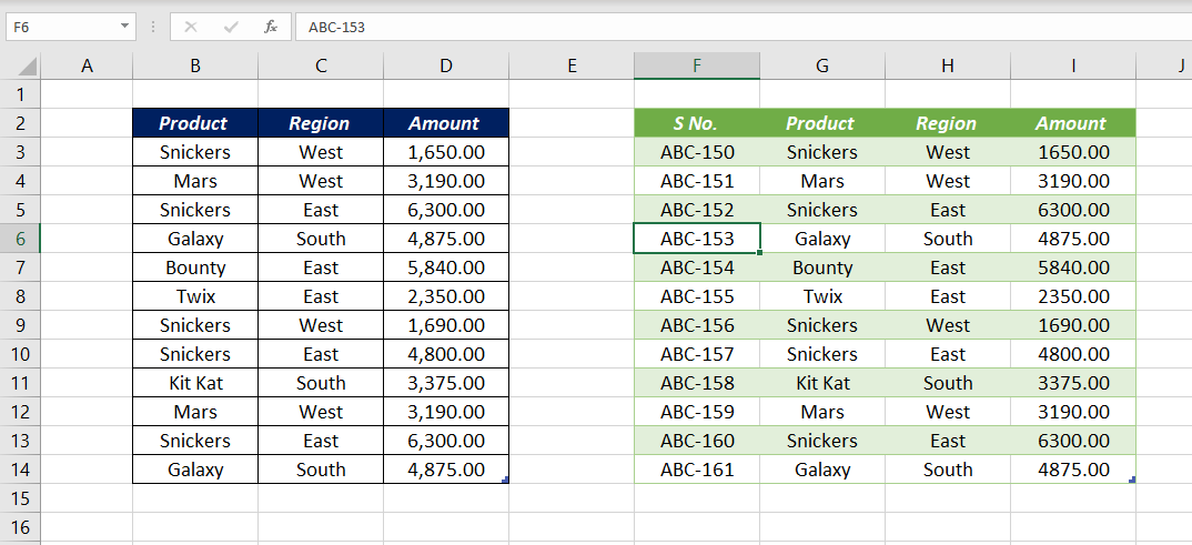
Now, if I want the Serial Number to start with a specific number like 150 or customize the Serial Number like ABC-150, here is how I would do that.
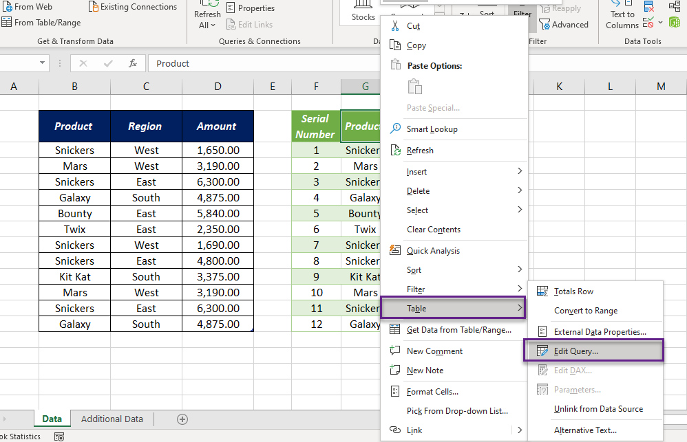
Right-click on the output table, Table > Edit Query
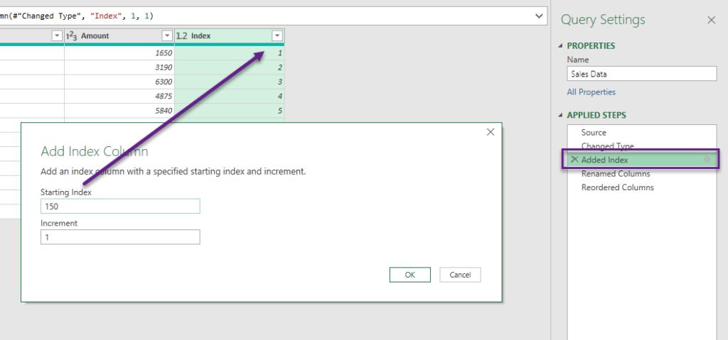
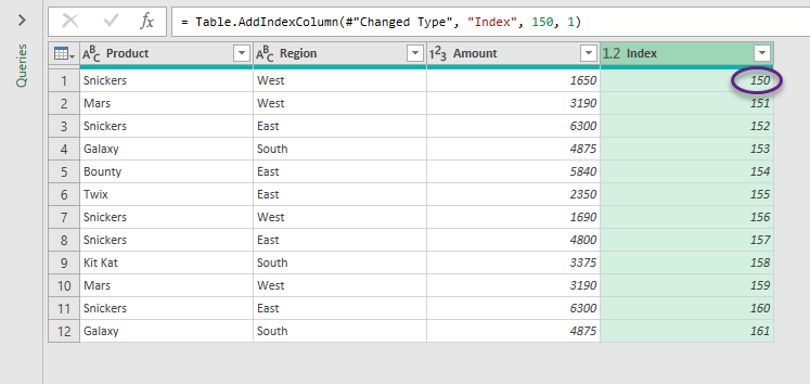
Power Query Editor will be activated. Double click on the Step called Added Index for the following dialog called Add Index Column.
For the serial number to start from 150, use 150 as Starting Index and Click OK. There is also an option for specifying the Increment.
Serial Numbers in the Index column have changed.
If you want to add some kind of Prefix or Suffix to these numbers,
In the Add Column tab > Format > select Add Prefix or Add Suffix
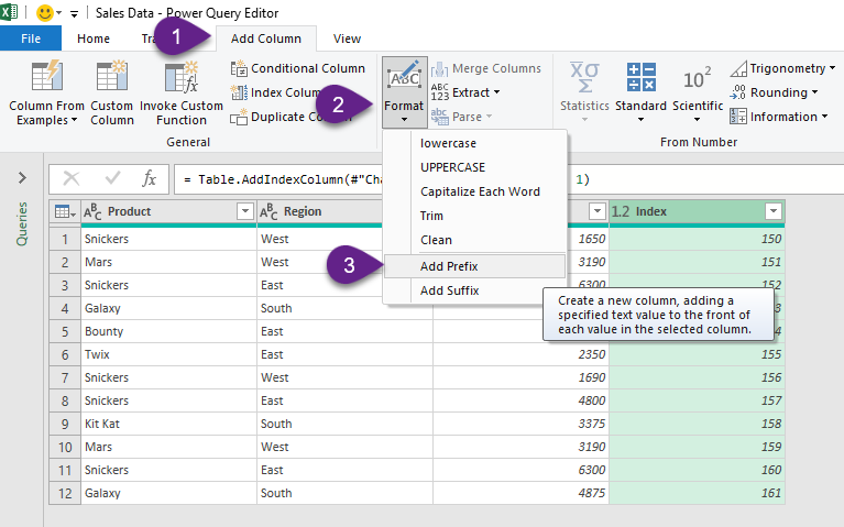
Here, I will be using the text ABC- as Prefix for the serial numbers.
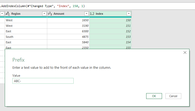
Type in ‘ABC-‘ in the input box under the label called Prefix and click OK
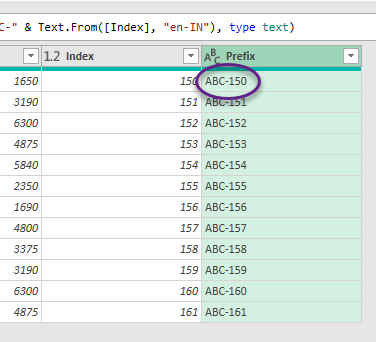
A new column is created which contains the Serial numbers starting from 150 and with a prefix ABC-
We need to make some changes to this query before loading it into the Excel sheet.
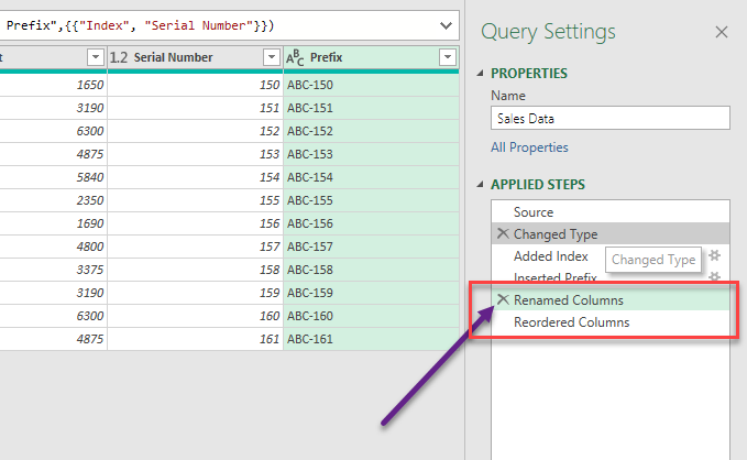
Click on the cross against the following two steps to delete them.
- Renamed Columns
- Reordered Columns
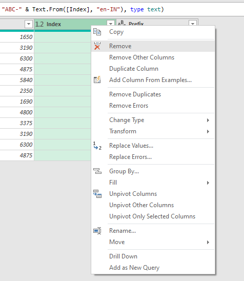
To remove the column called Index, Right-click on the Column header > select Remove
Rename the new column containing serial numbers as S No. and reposition it to the beginning of the data set.
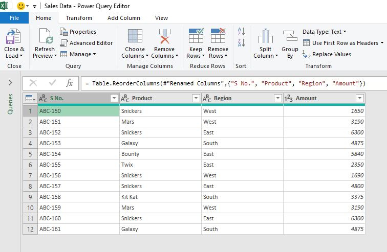
Click on Close & Load in the Home tab of Power Query Editor and the output table in the Excel worksheet will be updated like this.

Add some new data to the source table and refresh the Output table to see the Serial Numbers generated automatically.
If you are curious about the Formula method to generate Serial Numbers, I recommend the following video.