The Google Sheets QUERY function filters, sorts, totals and picks columns from a table in one formula, using simple words like select, where, group by and order by. Excel has no direct equivalent.
data |
The table including headers, such as A1:D9. |
|---|---|
query |
The instructions in double quotes, such as "select A, D where B = 'Kochi'". Columns are named by letter; text values go in single quotes. |
headers optional |
The number of header rows in data. Use 1. |
Basic example
To list the reps and amounts for Kochi only:
=QUERY(A1:D9,"select A, D where B = 'Kochi'",1)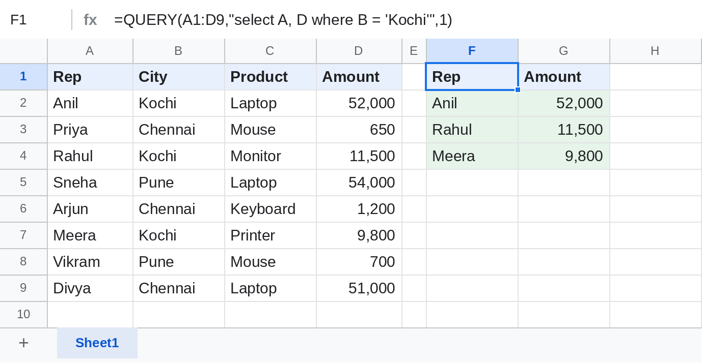
select A, D picks the Rep and Amount columns and where B = 'Kochi' keeps the Kochi rows: Anil, Rahul and Meera. The header row comes with the result.
Total by group and sort
=QUERY(A1:D9,"select B, sum(D) group by B order by sum(D) desc label sum(D) 'Total'",1)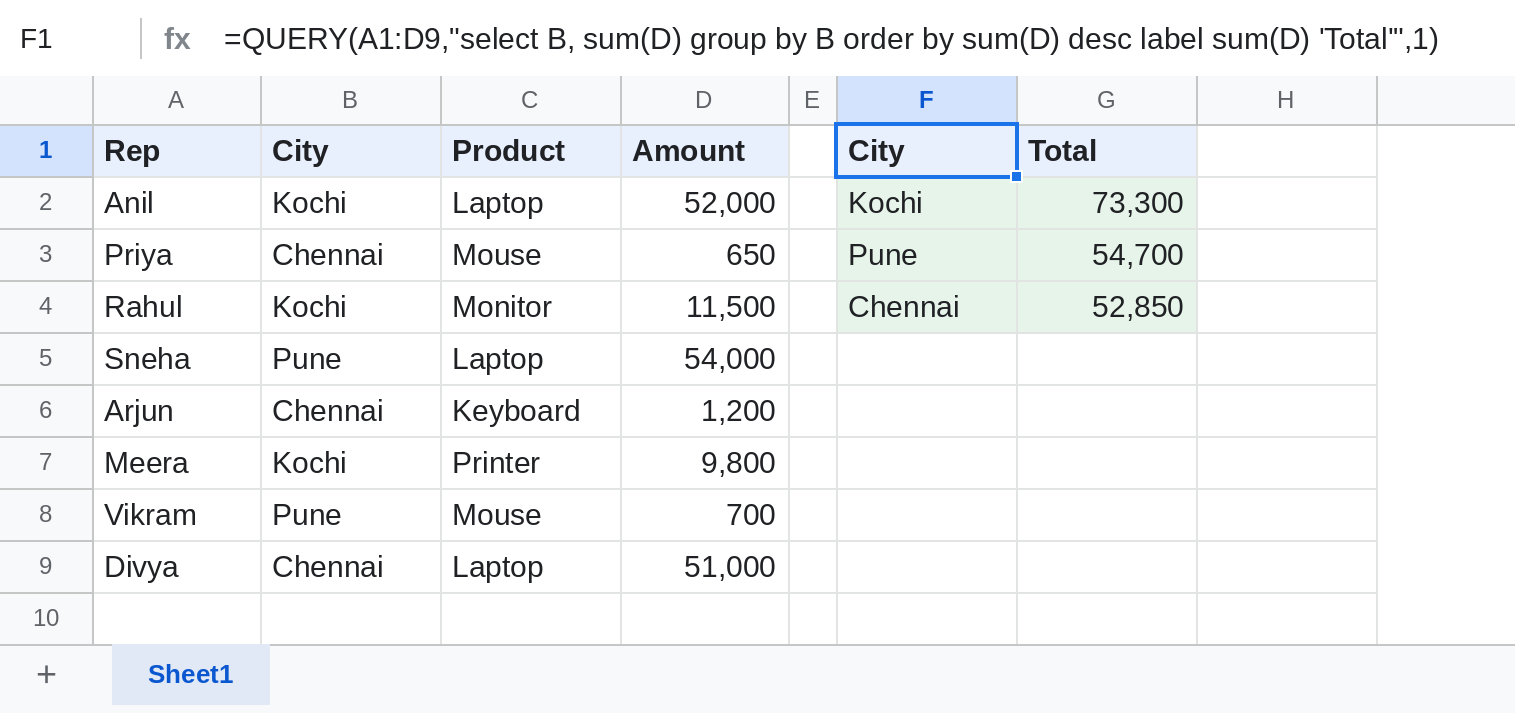
group by B gives one row per city, sum(D) totals each city, order by … desc puts the largest first and label renames the heading. Kochi leads with 73,300. It's a PivotTable in one formula.
Several conditions
=QUERY(A1:D9,"select * where C = 'Laptop' and D > 10000 order by D desc",1)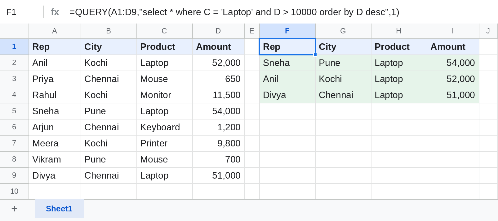
select * returns every column. Join conditions with and or or. Numbers take no quotes.
Use a cell in the condition
To pick the city from G1 instead of typing it into the formula, join the cell into the text:
=QUERY(A1:D9,"select A, D where B = '"&G1&"'",1)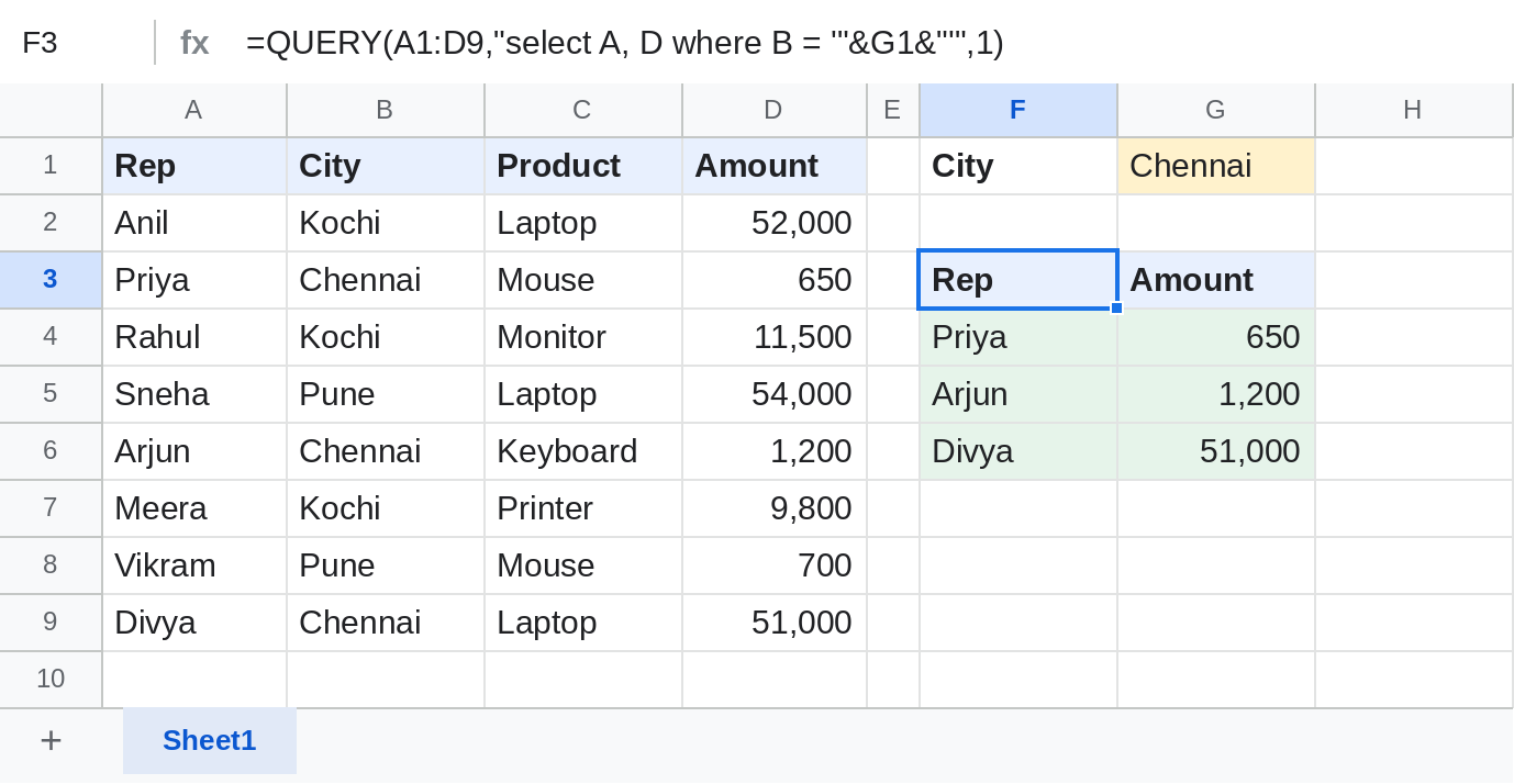
Change G1 to Pune and the result updates. For a number in a cell, leave out the single quotes: "where D > "&G1.
Query clauses cheat sheet
| Clause (in this order) | Example | Does |
|---|---|---|
| select | select A, D |
Chooses columns (* for all) |
| where | where D > 10000 |
Filters rows |
| group by | group by B |
One row per value, with sum, count, avg, max or min |
| pivot | pivot C |
Turns values into column headings |
| order by | order by D desc |
Sorts |
| limit | limit 5 |
Returns the first rows only |
| label | label sum(D) 'Total' |
Renames a heading |
| format | format D '#,##0' |
Formats a column |
Text tests: contains 'an', starts with 'P', is not null (skips blanks). Dates: where E > date '2026-10-01'.
Notes
- Clauses must be in the order shown in the cheat sheet, or QUERY returns an error.
- If a column mixes numbers and text, QUERY uses the type most cells have and shows the others as blank. Keep each column to one type.
- With IMPORTRANGE or
{}arrays as data, name the columnsCol1,Col2… instead of A, B.
Common errors
| Problem | Cause | Fix |
|---|---|---|
| #VALUE! Unable to parse query string | A typo, missing quote or clauses in the wrong order | Check the quotes and the clause order |
| #VALUE! NO_COLUMN | A column letter outside the data range | Use letters inside the range, or Col1, Col2 for arrays |
| Blank cells where numbers should be | The column mixes text and numbers | Make the column one type |
| #REF! | The result would overwrite cells | Clear the cells below and to the right |
Practice file
The sales table with all four QUERY examples working. Upload it to Google Drive and open it with Google Sheets.