How to build Relationships between Excel Tables using the Data Model of Excel is explained in this Tutorial.
Table of Contents
Purpose of connecting Tables
VLOOKUP and INDEX+MATCH formulas always get the job done, but a lot of them will essentially slow down the workbook. Moreover, the Lookup and Reference formulas also demands maintenance with addition or deletion of data.
Excel’s Data Model which was introduced with Excel 2013, allows us to connect Tables using which, we can avoid the pain of creating complex Lookup and Aggregate formulas.
Let me show you an example for the need of connecting Tables and after that we will go through the step by step procedure of building relationship.
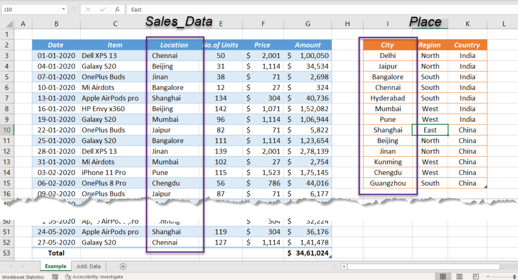
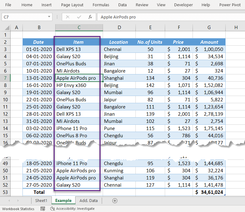
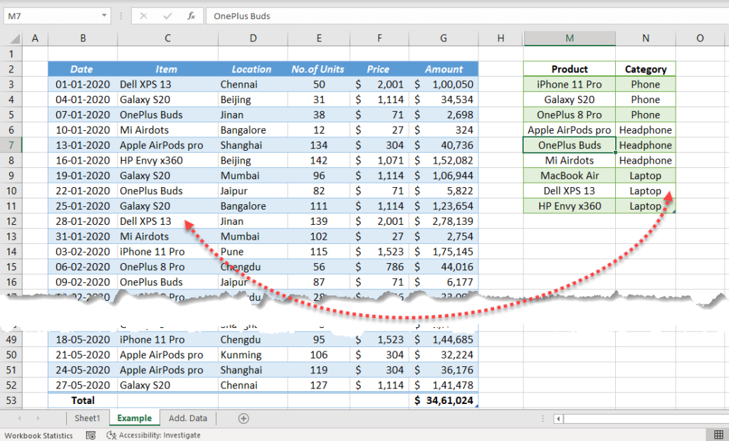
Following is the sales records of a particular company which deals with the sale of electronic gadgets in different parts of India and China. This table called Sales_Data contains 6 columns which are for Date, Product Name, Location of sale, Number of units sold, Unit price of the product and Amount.
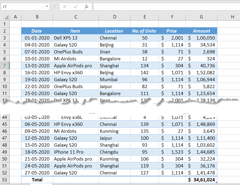
Now, one of the company managers wants to know the Total Sum of Sales done in the Southern part of India.
Total Sum of Sales in the South Region of India?
As you can see, the table for sales records doesn’t have the details of Region or Country. There is only one column that has the information about the place of sale, the column called ‘Location’ which contains the name of the city.
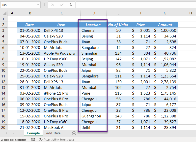
The details regarding cities i.e. corresponding Region and Country are in another Table called Place.

Now that we have the required details in two different tables, how can we find the Total Sum of Sales done in the South Region of India?
Solution 1 (Using VLOOKUP function and Pivot Table)
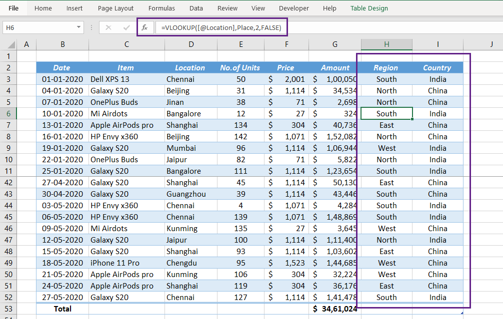
One of the different methods to solve this problem is creating two new columns for corresponding Region and Country in the source data using VLOOKUP function.
Then summarize the data using a Pivot Table for the required figure.
The drawbacks of this method are…
- Source data will be disturbed.
- For 50 records, we should create 100 new VLOOKUP formulas. (For bigger data sets, these additional formulas will affect the calculation speed of the workbook)
- If a new question arises, maybe for the Total sum of sales for Phones or Laptops we need to add more columns and formulas.
Solution 2 (Using VLOOKUP and SUMIFS functions)
Create columns for corresponding Region and Country outside the source data using VLOOKUP function.

Apply SUMIFS function for the ranges containing Region and Country with ‘South’ and ‘India’ as criteria.
=SUMIFS(Sales_Data[Amount],I3:I52,"South",J3:J52,"India")

Here we aren’t touching the source data, but as you can see the procedure is lengthy and creating 100 more formulas. The solution demands the command over VLOOKUP and SUMIFS functions and for additional queries we may need to create more columns and formulas.
Solution 3 (By connecting Excel Tables)
The most elegant solution to this problem which won’t disturb the source data is establishing a relationship between the Excel tables Sales_Data and Place. Once these tables are connected we can create the Pivot Table Reports of our choice.
Requirements for building relationship between tables
- The primary requirement to connect two Excel Tables is, both of these tables should contain at least a ‘column with common values‘. Here both the tables have a column in common, the columns containing the name of Cities.
- The second requirement is one of these columns containing common values shouldn’t have any duplicates. Here that requirement also is satisfied. The column called City of the table called Place doesn’t have any duplicates.
Now that both the requirements are satisfied let’s connect the tables Sales_Data and Place.
Go to the Data tab of Excel ribbon > Click on the Relationships button in the group called Data Tools to activate the dialog called Manage Relationships
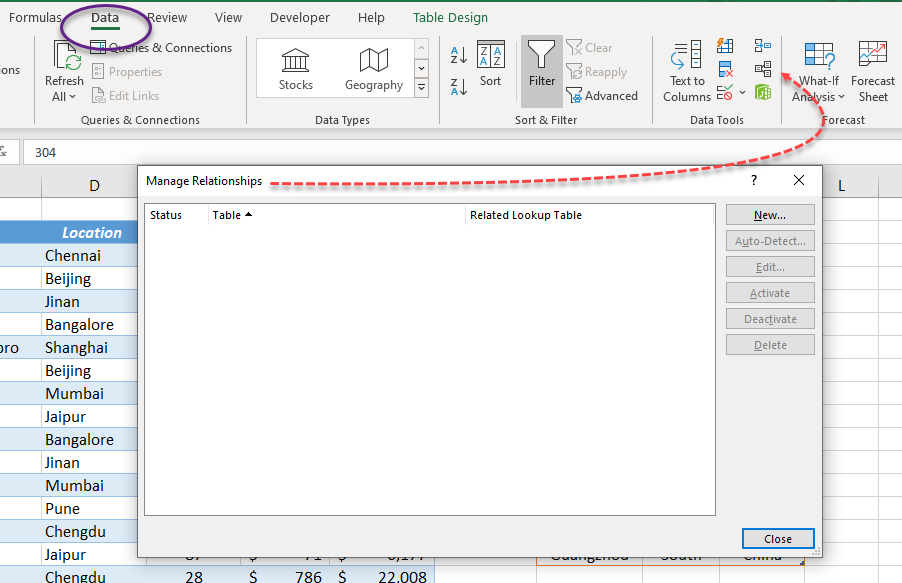
Click on New and we will have another dialog called Create Relationships. The drop down menus in this dialog can be used to select the ‘Tables’ and corresponding ‘Columns’ to connect.
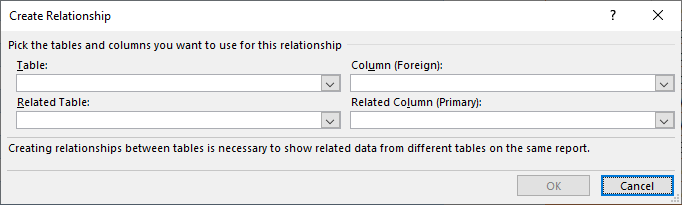
Table will be that table containing the source data or in other words the bigger table.
Foreign column is the column containing common values. In this case Sales_Data will be the Table and the column called Location will be the Foreign column.
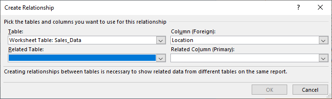
Related Table will be the table containing that column without duplicates.
Related Column will be the column containing common values. In this case Place will be the Related Table and the column called City will be the Related Column.
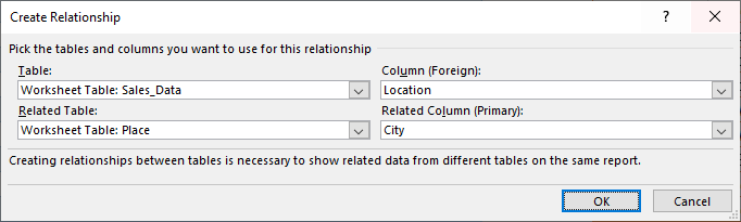
After selecting the tables and corresponding columns, click OK to create the connection.
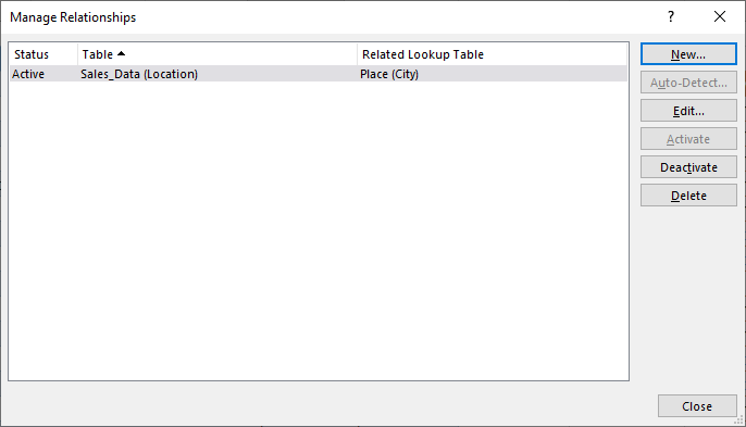
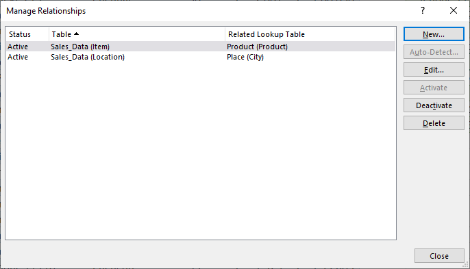
Once the connection is established, these tables will be loaded to the Data Model of the workbook and the connection will be listed in the Manage Relationships dialog.
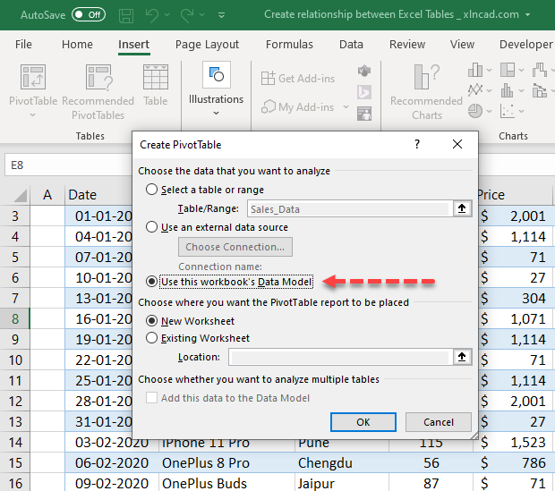
To create a Pivot Table report using this data,
Go to the Insert Tab > Pivot Table > Use this workbook’s Data Model > OK
Both the tables Sales_Data and Place are listed in the field list of the new Pivot Table.
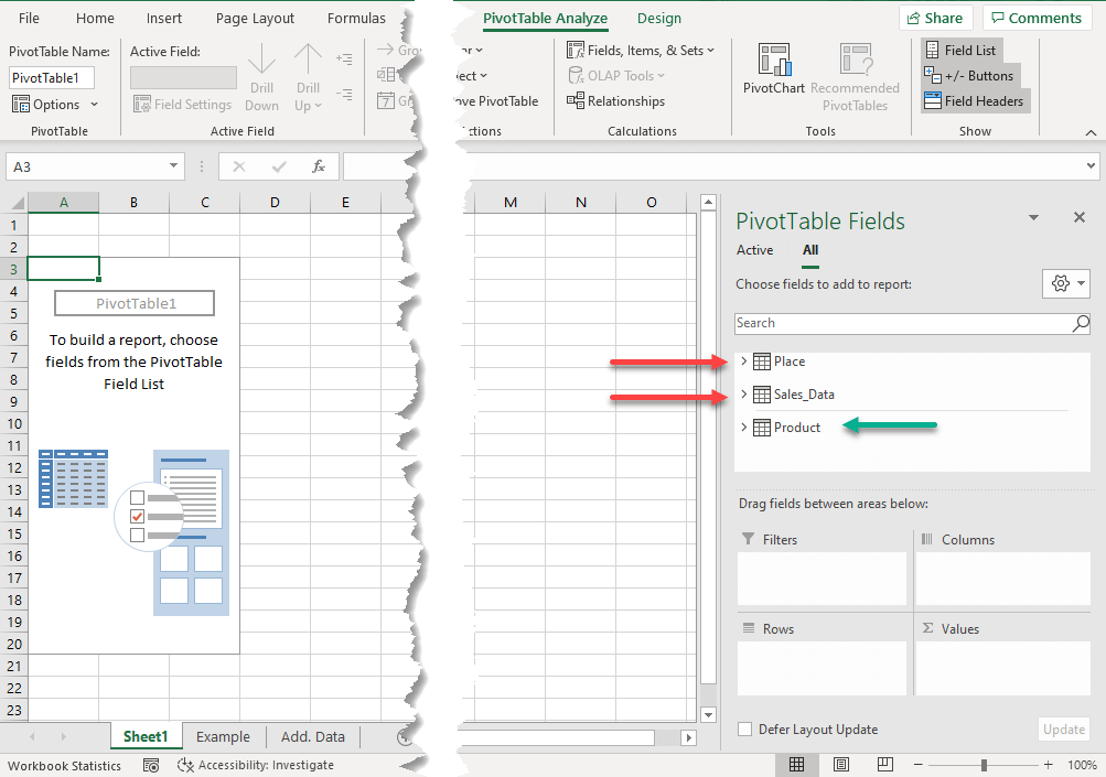
Product is another table available in the workbook and as you can see a thin line is separating this label from the related tables.
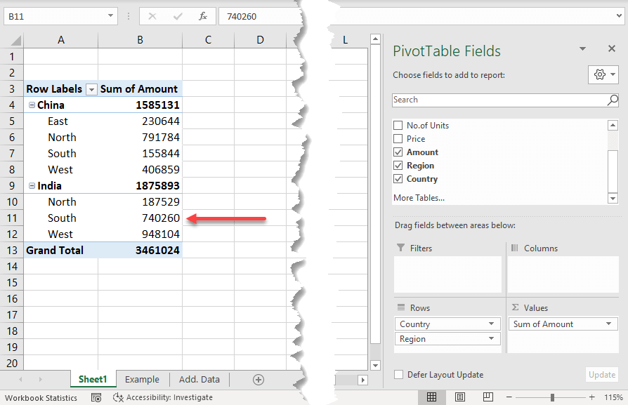
For the Region wise Sum of Sales,
Drag and drop the fields called Region and Country into the ‘area for Rows’ and the field called Amount into the ‘area for Values’.
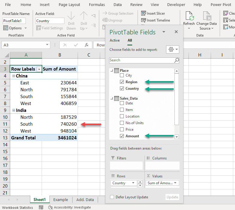
Sum of Sales for South region of India is 740260.
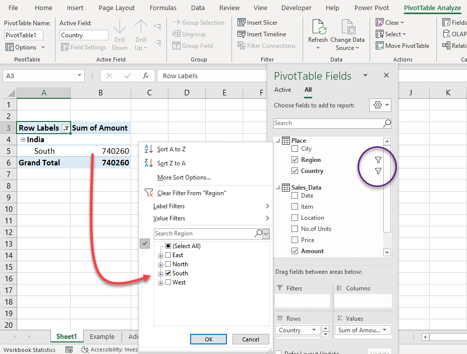
To remove other values, apply filter using the filter buttons against the fields, Region and Country.
Connecting more Tables
As soon as we solved the first question, another manager wants to know the Count of Cell phones sold in the East and West regions of China.
Total number of Cell phones sold in the East and West regions of China?
As you can see below, the table called Sales_Data has a column for item but it doesn’t have the details of categories. i.e. the table doesn’t say whether an item is a Phone, Laptop or Headset.
The details regarding each item i.e. corresponding Category is in another Table called Product.
This question is more complex than the previous one and if you try to solve it using VLOOKUP function, it will take 3 VLOOKUP formulas (Region, Country and Category) for each record. i.e. 150 VLOOKUP formulas for 50 records.
As Excel doesn’t limit us from creating multiple relationships between multiple tables, this question can be easily solved by connecting the source data with the table Product.
To connect the tables, Sales_Data and Product,
Activate the Manage Relationships dialog from the Data tab of Excel Ribbon > New > In the dialog for Create Relationship, specify the tables and columns needed for creating relationship.
Sales_Data will be the Table and the column called Item will be the Foreign column.
Product will be the Related Table and the column called Product in that table will be the Related Column.
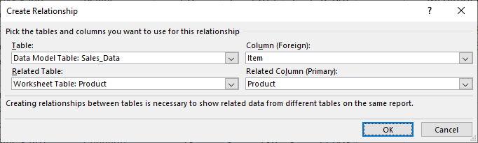
Click OK and the new relationship will be listed in the Manage Relationships dialog.
Now that the 3 tables are connected we can find out the Count of Phones sold in the East and West regions of China either by modifying the existing Pivot Table or by creating a new one.
For the Total number of Phones sold in the East and West regions of China,
Drag and drop the fields for Region, Country, Product and Category into the area for Rows and the field called No. of Units into the area for Values.
Apply the corresponding filters for ‘China’, ‘East’, ‘West’, ‘Phone’ and we will have the Total number of phones sold in the East and West regions of China.
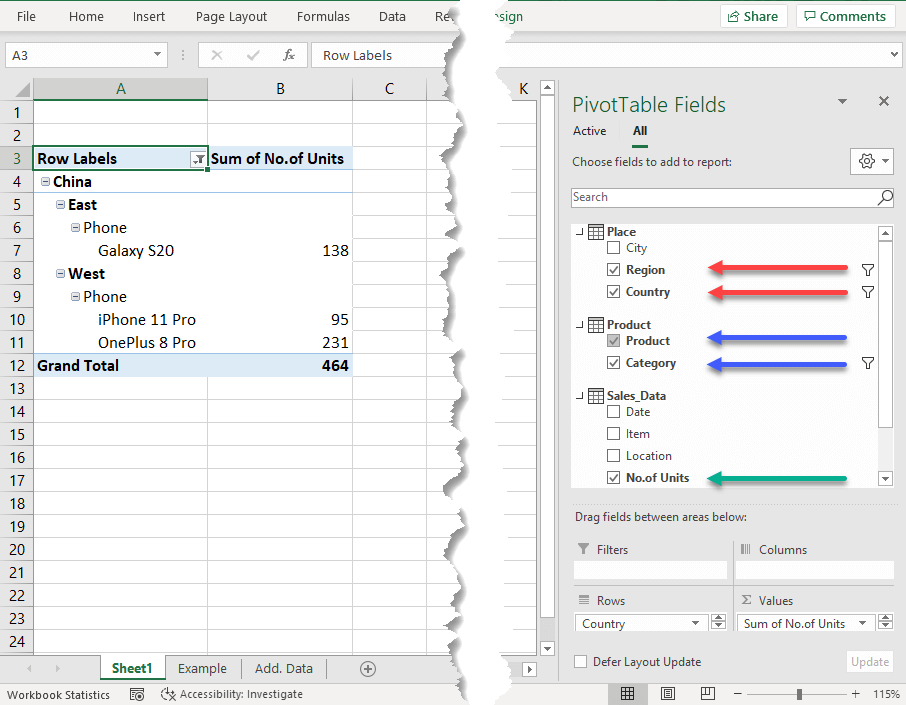
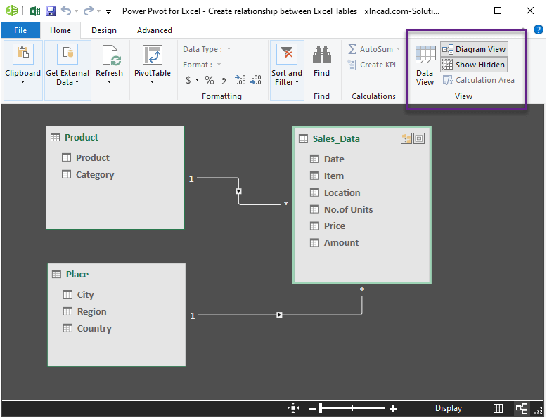
Diagram View of Relationships
Following is the diagram view of the relationships that we created between the Tables Sales_Data, Place and Product. The same can be activated from the Home tab of Power Pivot window.
Notes:
- Data model is only available to Excel 2013 and later versions.
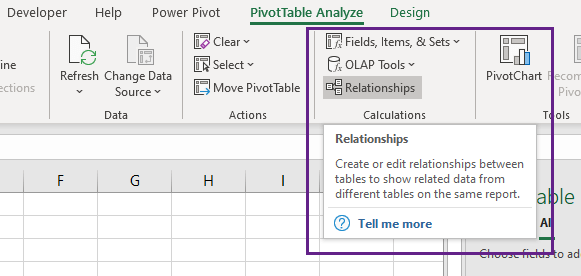
- Manage Relationships dialog can also be activated from the PivotTable Analyze tab of Excel Ribbon.