Drop-down list in Excel

Table of Contents

Create a Drop-Down List

A drop-down list, also known as a drop-down menu is a graphical control object that offers a list of options. In cells with a drop-down list, the user need not type in anything but can make the selection from the available options.

In this blog post you will see, How to set up a Drop-down list using the Data Validation feature in Excel.

Following is a list of Indian desserts (cells from B3 to B6).

To create a drop-down list of the above desserts in a cell or cells,

Select the cell or cells where you want the drop-down list. In the Data tab of Excel Ribbon > Data Tools > Data Validation

In the dialog called Data Validation > Settings > Select ‘List’ from the options under the heading Validation criteria

In the Input box under the heading ‘Source’, either type in the address of the cells containing the source data or select those cells using the mouse.

In this case, B3:B6 is the address of the cells containing source data. $ is added before the Row and Column indexes to make the references ‘Absolute’.

Click OK and you will have a drop-down list in the selected cell/cells. A cell with a drop-down list, when selected will display a small down arrow on its right side.

Drop-down list of that cell can be activated by clicking this arrow or the keyboard shortcut, Alt + ↓

Drop-down list can be copied to other cells using the Excel ‘fill handle’ or the Copy-Paste option.

Also, if you try to make an entry that is not listed in the drop-down list, Excel will display a warning message.

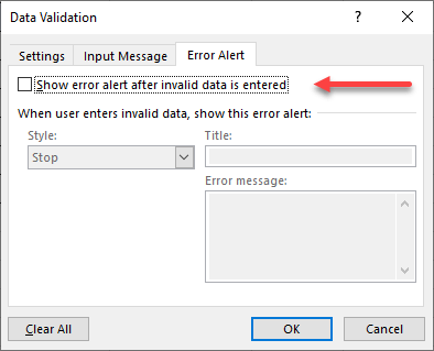
To allow values other than those listed in the drop-down menu,

Activate the Data Validation dialog > In the Error Alert tab, unmark the checkbox against the label, ‘Show error alert after invalid data is entered’.

Drop-down lists with manually entered data

Drop-down menus can also be created using manually entered data. Suppose you want a drop-down list with only two options Yes and No…

Select the cell or cells where you want the drop-down list and activate the dialog for Data Validation from the Data tab.
In the dialog called Data Validation > Settings tab > Select ‘List’ from the options under the heading Validation criteria
In the Input box under the heading ‘Source’, type in ‘Yes, No’

Click OK and we will have a drop-down list with two options ‘Yes’ and ‘No’ in the selected cell/cells.

Dynamic drop-down list

The drop-down lists which we created in the above examples are of static nature. If you want to add data to the lists like these, you should update the source data as well as the address of the source specified in the Validation criteria.

There are a few ways to make a drop-drop list dynamic and the easiest one is converting the source data into an Excel Table.

Select the cells containing data > go to the Insert tab in the Excel Ribbon > Table > Click OK

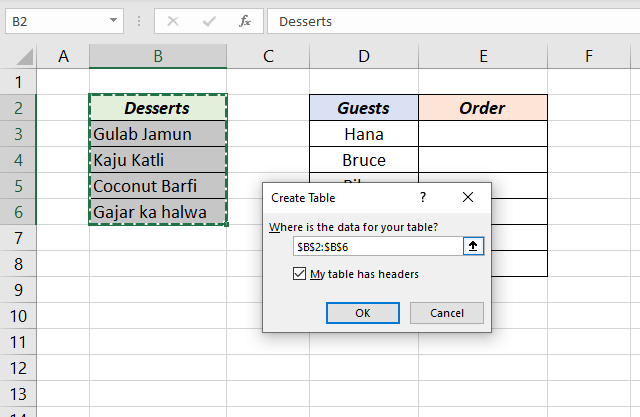
Ctrl +T‘ is the keyboard shortcut to create Table in Excel

After converting the data into Excel Table, I have named it as ‘Food’.

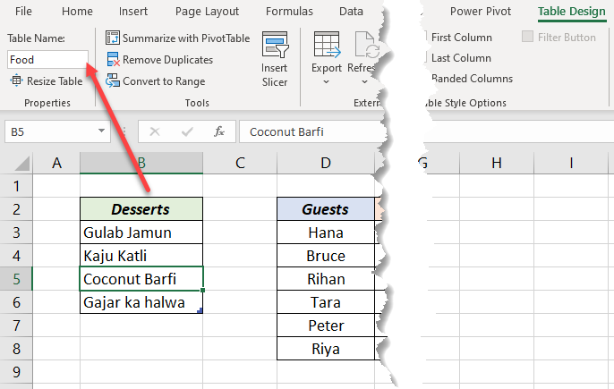
To use this table as source data of a drop-down list,

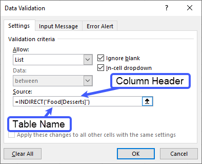
Select the cells where you want the drop-down list > Activate the Data Validation dialog > Select List from the Validation criteria > Type in the following formula in the input box for Source