
Conditional Formatting in Excel can be used to shade alternate Rows or Columns. Another method is converting the Data set into an Excel Table. This method should be adopted if your dataset is supposed to expand.
Method 1: Conditional Formatting for shading alternate Rows
Suppose we have a dataset like the one shown below.

To highlight alternate rows of this dataset in Blue color, select the data
Go to Conditional Formatting > New Rule > Use a formula to determine which cells to format and Type in the following formula
=MOD(ROW(),2)
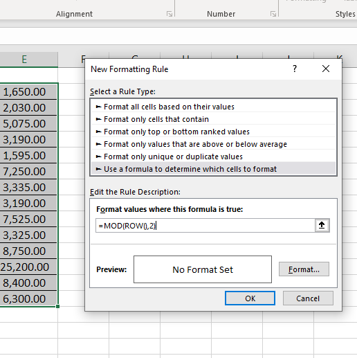
Click on Format… > Select the desired background color (I have selected Blue color) from the Fill tab of the Format Cells dailog > Click OK

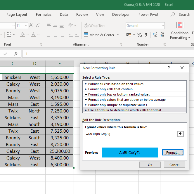
Now, the New Formatting Rule dialog has the preview of the formatting to be applied. Click OK to confirm.
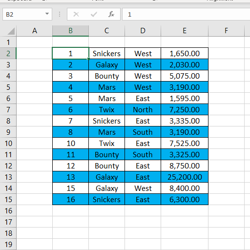
Alternate cells of the selected data are now highlighted in Blue color
Method 2: Highlight alternate Rows of a dataset by converting it into an Excel Table
To convert the dataset into an Excel Table,
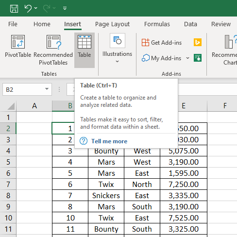
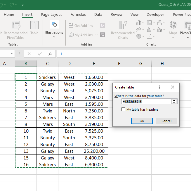
Select a cell in the dataset > Go to Insert Tab > Click on Table
Create Table Dialog will be activated > Click OK to create the table.
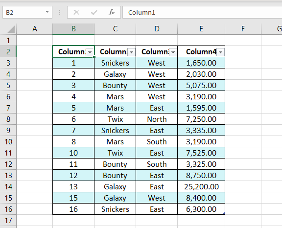
Selected data is now converted into an Excel Table and the alternate rows are highlighted.
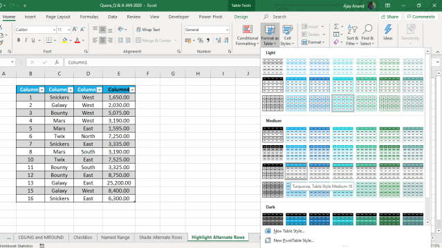
To use a predefined style or to create a new style use the Format as Table option in the Home tab of Excel Ribbon.
Read about
Conditional Formatting in Excel