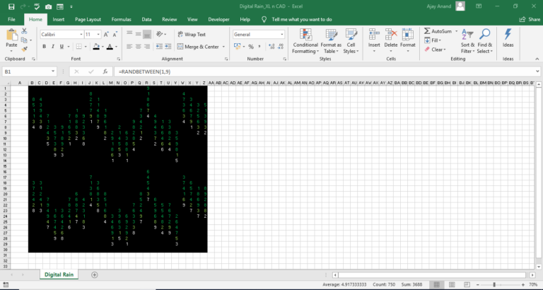
I hope you will be familiar with this visual effect from the classic SCI-FI movie Matrix. This effect is known in different names like Matrix code rain, Matrix Digital rain, etc. What you see here is an animation created in an Excel Sheet using Conditional formatting, RANDBETWEEN function, and a simple macro.
The idea was originally conceived by Mr. Nitin Mehta of XLnControl Pty Ltd. My contribution is adding a macro to automate the process. Read about the original version here at Engineers-Excel.com
Now, let’s see how to create this animation.
Like I mentioned above, there are 3 major components used in creating this Visual effect in Excel.
1. First component is RANDBETWEEN function.
RANDBETWEEN function is used to return a random number between the Bottom and Top limits specified inside the function.
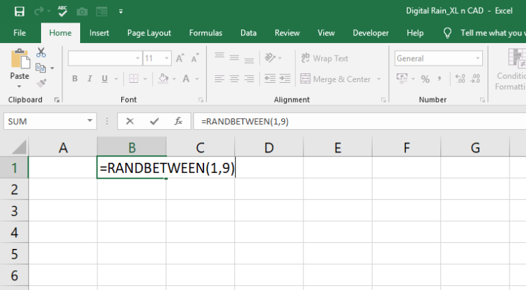
Select the cell B1 and type in the following formula
=RANDBETWEEN(1,9)
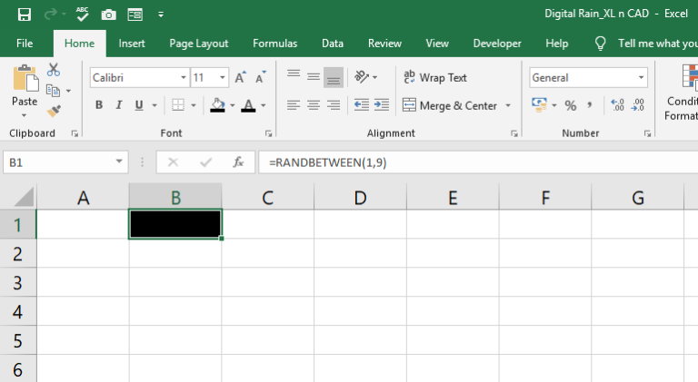
Change the background Color and font Color of the cell B1 to Black
2. The Second and Major component is CONDITIONAL FORMATTING.
Click on Conditional Formatting in the Home Tab
Select New Rule
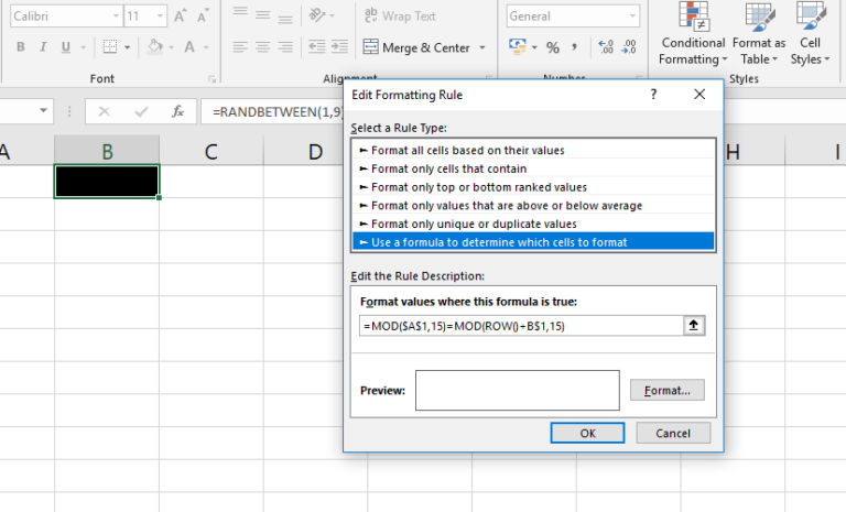
Select the option called Use a formula to determine which cells to format and use the following formula
=MOD($A$1,15)=MOD(ROW()+B$1,15)
Click on Format and change the font color to WHITE
And following is the explanation to the formula
MOD function is used to return the Remainder after dividing a number with a divisor. For example, =MOD(10,3) will return 1. Here 10 is the Number, 3 is the Divisor and 1 is the Remainder.
ROW function is used to return the Row Number of a cell reference. For example, ROW(H7) will return the value 7 since H7 is in the 7th Row of the worksheet.
Suppose the cell A1 is having the value 13, B1 – 8, J1 – 5 and the cell J8 is having the value 4
And when we use the formula = MOD($A$1,15)=MOD(ROW()+B$1,15) in the cell B1, the formula will be evaluated to
=MOD(13,15)=MOD(1+8,15)
=13=9
=FALSE
As the condition turned out to be false, font color will be black and the content in the cell B1 won’t be visible.
and when the same formula is used with the cell J8, will be evaluated to
=MOD(13,15)=MOD(8+5,15)
=13=13
=TRUE
As the condition turned out to be TRUE, font color will be WHITE and the content in the cell J8 will be displayed in white
Copy this formula as we will be using this formula a few times more.
Click Ok to close the dialogue box
Once again, Click on conditional Formatting
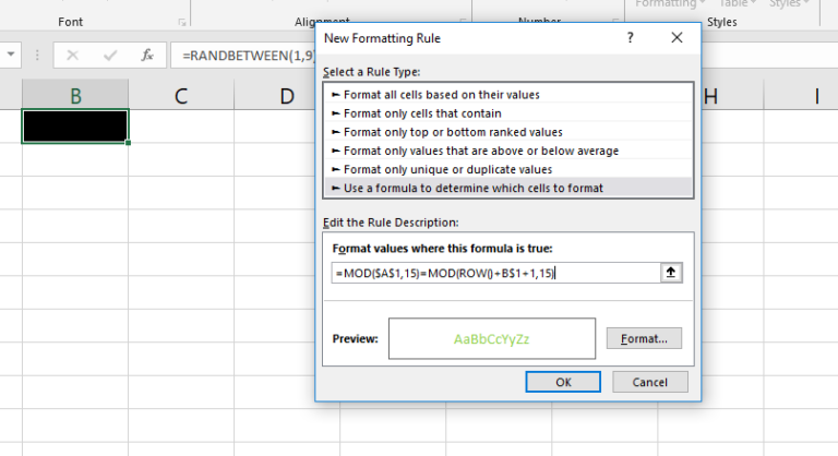
Click on new rule, select the option the option called Use a formula to determine which cells to format, and Paste the copied formula
Modify the formula to =MOD($A$1,15)=MOD(ROW()+B$1+1,15)
Click on format and change the font color to BRIGHT GREEN
And following is the explanation to the formula
This formula will set the font color of the number just above the white number to bright green.
We have seen the first formula was evaluated as TRUE for the cell J8 and the font color became white for the cell J8
=MOD($A$1,15)=MOD(ROW()+B$1+1,15) for the cell J7 will be evaluated as
=MOD($13,15)=MOD(7+5+1,15)
=MOD($13)=MOD(13)
=TRUE
As the condition turned out to be TRUE, the content in the cell J7 will be displayed in Bright Green.
Click OK to close the dialogue box
Now the third and last rule for conditional formatting
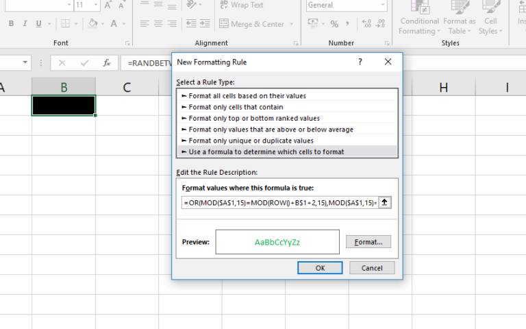
Click on Conditional Formatting, Select new rule and add type in the following formula
=OR(
Paste the copied formula 4 times with a comma between
Modify B&1 in each segment to B$1+2, B$1+3, B$1+4 and B$1+5 so that the final formula will be
=OR(MOD($A$1,15)=MOD(ROW()+B$1+2,15), MOD($A$1,15)=MOD(ROW()+B$1+3,15), MOD($A$1,15)=MOD(ROW()+B$1+4,15), MOD($A$1,15)=MOD(ROW()+B$1+5,15))
Click on Format and change the font color to DARK GREEN
And following is the explanation to the formula
This third formula is to create a dark tail of 4 cells to follow the bright green cell.
We have seen the first formula was evaluated as TRUE for the cell J8 and the font color became white, the second formula was evaluated as TRUE for the cell J7 and the font color became bright green
=OR(MOD($A$1,15)=MOD(ROW()+B$1+2,15), MOD($A$1,15)=MOD(ROW()+B$1+3,15), MOD($A$1,15)=MOD(ROW()+B$1+4,15), MOD($A$1,15)=MOD(ROW()+B$1+5,15)) for the cell J6 will be evaluated as
=OR(MOD(13,15)=MOD(6+5+2,15), MOD(13,15)=MOD(6+5+3,15), MOD(13,15)=MOD(6+5+4,15), MOD(13,15)=MOD(6+5+5,15))
=OR(13=13,13=14,13=15,13=16)
=OR(TRUE,FALSE,FALSE,FALSE)
=TRUE
As one of the 4 conditions turned out to be true, the font color will be Dark Green. The cells J5, J4 and J3 will be having the same formatting due this formula. i.e. if you need a tail of 5 cells, add MOD(($A$1,15)=MOD(ROW()+B$1+6,15)) to the formula with a comma in between.
When none of these conditions are met, the content in the cells will be invisible as the default font color of the cell is black.
Reduce the column width so that the animation will look better
Copy the cell B1 and paste it into the adjacent cells
Copy the first row and Paste As Values into the same row
And we are almost done with random numbers in different colors
3. Now the third component and last component, A Macro which will trigger the code fall
Click on Visual Basic in the developer tab
Right click on the tree view on the left sidebar and Insert a module
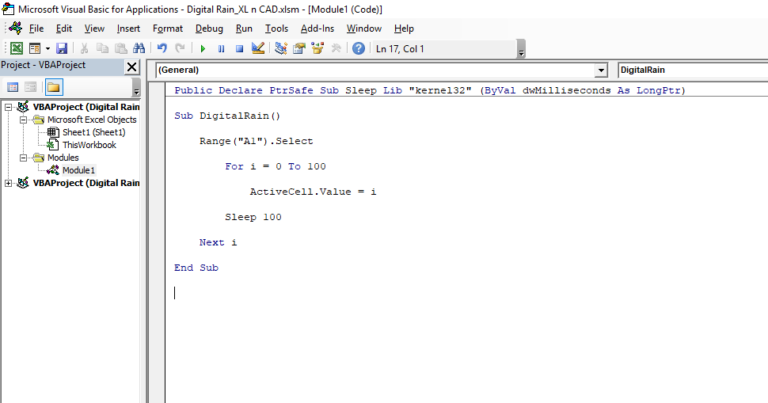
Type in the following code or you can copy this code as it is. Please note that the statements which start with an apostrophe won’t have any effect in the code. The explanations to each statement in the code and are known as comments.
Public Declare PtrSafe Sub Sleep Lib “kernel32” (ByVal dwMilliseconds As LongPtr)
Sub DigitalRain()
‘DigitalRain is the name of the macro
Range(“A1”).Select
‘This statement is to select the cell A1. After this statement A1 will become the activecell. i.e the cell where the control is
For i = 0 To 100
‘For loop is used for incrementing the value in the cell A1. ‘i’ is a variable used to store value.
ActiveCell.Value = i
For each iteration of the loop, value in the activecell (A1) will become same as that of the value of i
Sleep 100
This statement is used for a delay in executing the code. Otherwise, the code will execute in a pace in we won’t able to see the animation. 100 means 100 milliseconds
Next i
End Sub
Back to the sheet and insert a button from the Form control
Assign the button with the Macro, Digital Rain.
Click on the button to see the magic!