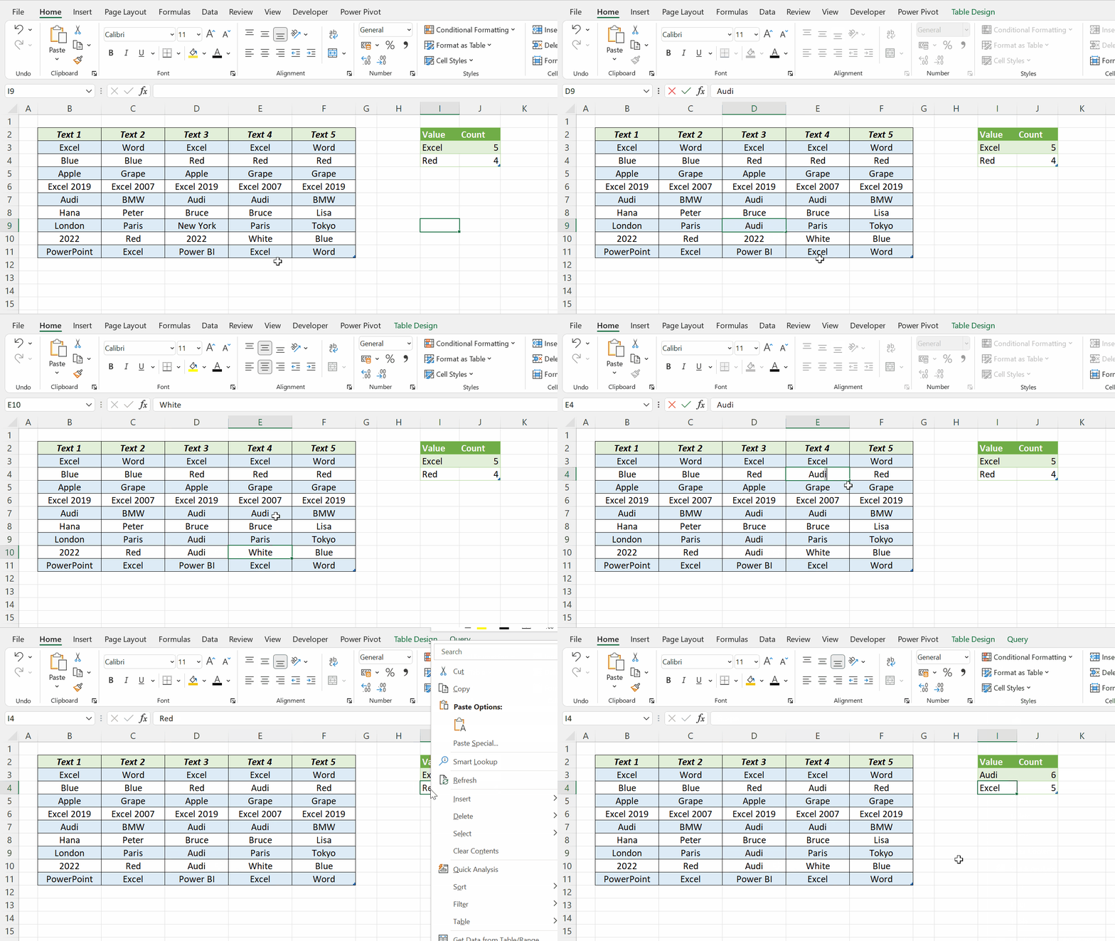
This blog post is about different ways to find the ‘Most Repeated Number or Text’ in a data set.
Table of Contents
Formula to find the most repeated Number
The MODE function in Excel is designed to return the most repeated number from a numeric dataset.
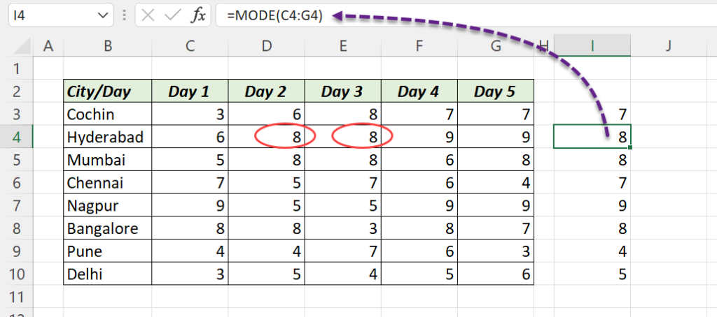
An example with vertical data ranges.
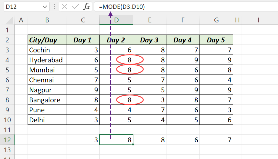
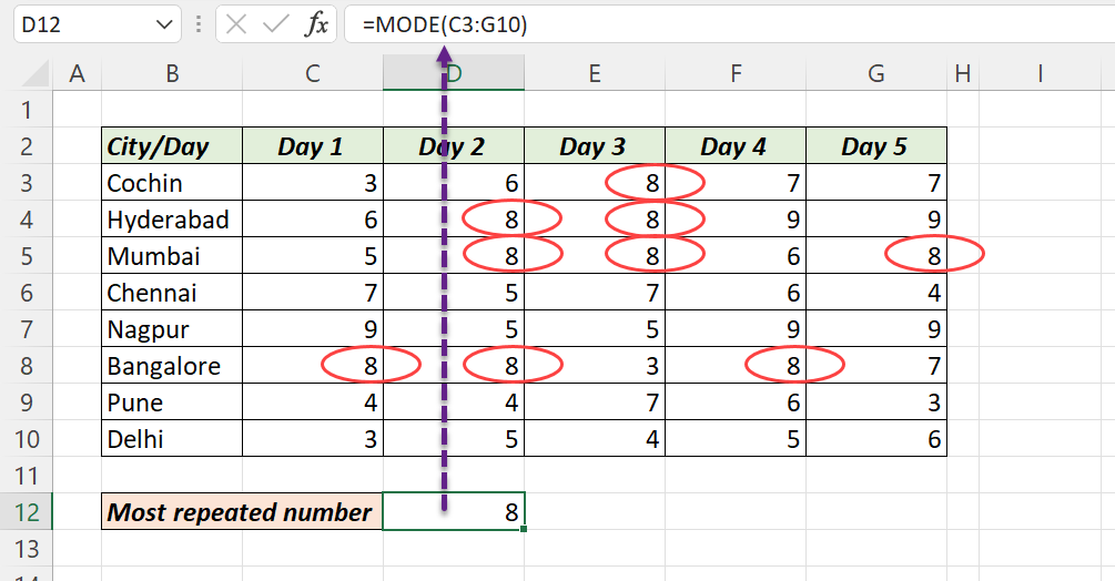
Another example with a 2 dimensional data range.
The MODE function returns 8 which is the most repeated number in the data range, C3:G10.
Excel process Date and Time as Numbers. So, the MODE function can also be used to find the most repeated Date from a set of Dates.
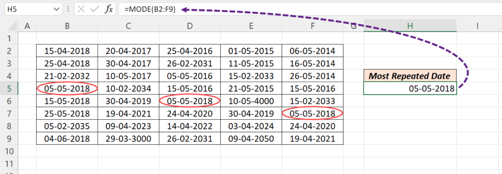
Formula to find the most repeated Text
The following formula will return the most repeated value in the range B5 to F5.
=INDEX(B5:F5,MODE(MATCH(B5:F5,B5:F5,0)))
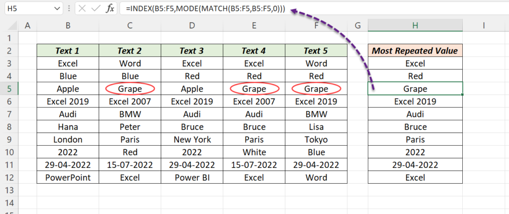
Note: The formula shown above is an Array formula. So, those who are using the Excel versions other than Microsoft 365 should enter this formula with the aid of ‘Ctrl + Shift + Enter’ keys
Explanation of the formula
=INDEX(B5:F5,MODE(MATCH(B5:F5,B5:F5,0)))
In the above formula, the lookup_value and lookup_array supplied into the MATCH function are the same.
=MATCH(B5:F5,B5:F5,0)

=MATCH({"Apple","Grape","Apple","Grape","Grape"},{"Apple","Grape","Apple","Grape","Grape"},0)
Means, the array {Apple, Grape, Apple, Grape, Grape} will match against itself and will return the result, {1, 2, 1, 2, 2}
Apple is in the 1st position of the array and whenever the MATCH function finds the word Apple, 1 is returned. Grape is in the 2nd position and the value 2 will be returned against Grape. So the resulting array will be {1, 2, 1, 2, 2}.
The MODE function will process this array and will return the most repeated number in this array, which is 2.
=MODE({1,2,1,2,2}

=2
The INDEX function will use process this value and will return the second element from the array supplied to it, which is Grape.
=INDEX({"Apple","Grape","Apple","Grape","Grape"},2))

="Grape"
Power Query to find the most repeated value
Power Query in Excel also can be used to find the most frequently occurring text in a data range.
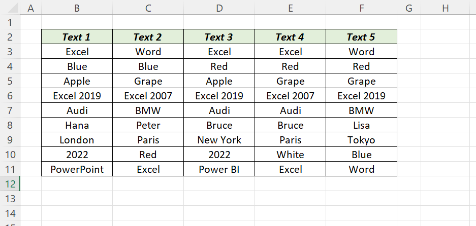
Suppose, we want to find the most repeated text in the following dataset.
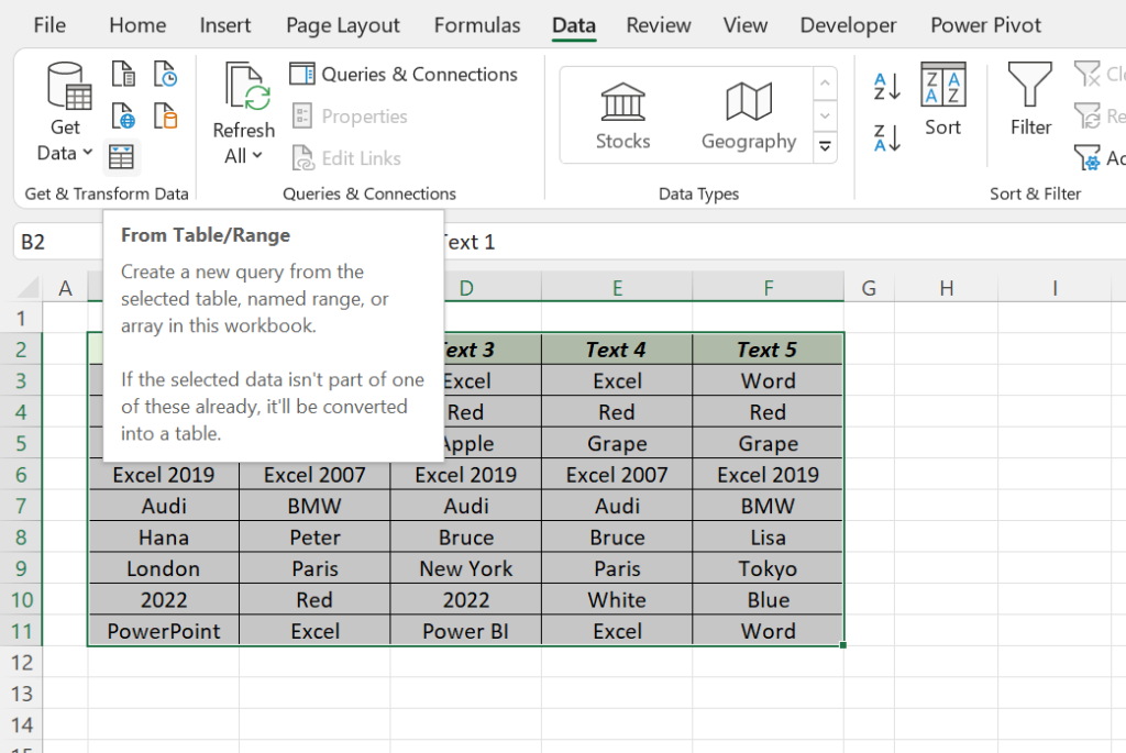
Select the cells containing data > go to the Data tab of the Excel ribbon > From Table/Range
If the selected data is not an official Excel Table, we will be prompted to convert it into a Table.
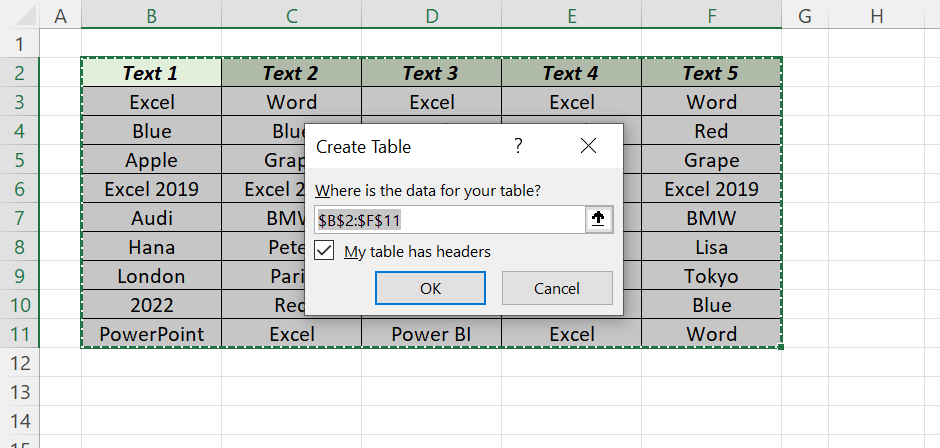
Click OK and the 5 columns of data will be loaded into the Power Query Editor of Excel.
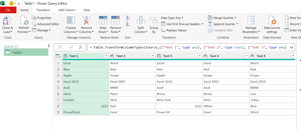
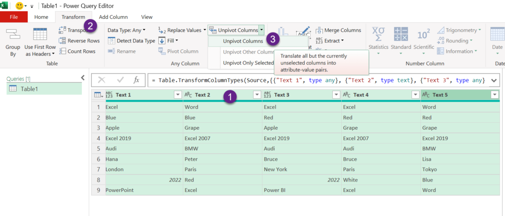
Next step is to bring all text values into a single column. For that,
select all columns > go to the Transform tab of the Power Query Editor > Unpivot Columns
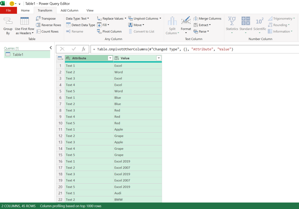
All text values will be stacked into a single column called Value.
Next step is grouping of Text and Numeric values. For that,
select the column containing Values > click on Group By
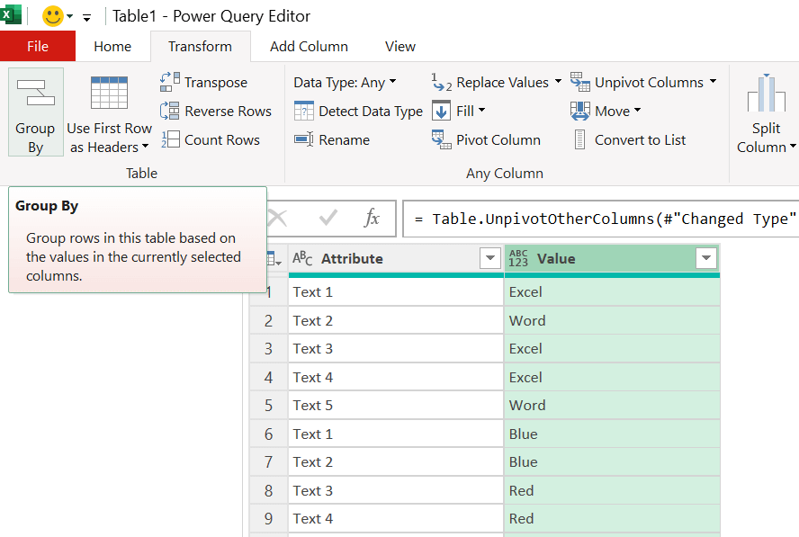
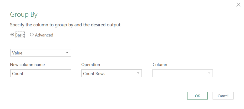
A dialog called Group By will be activated. This dialog can be used to specify the type of grouping Operation to be performed. In this case, we need the count of the Text values. So the Operation should be Count Rows.
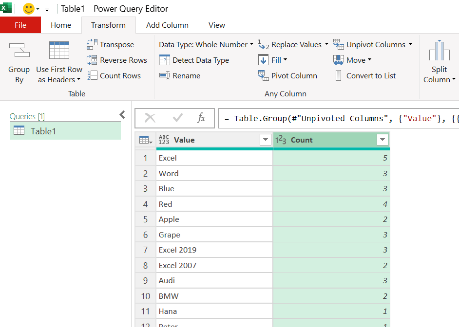
Click OK and a new column is created which contains the Count of each Value.
To sort this data in the descending order of Count,
select the column containing Count > go to the Home tab > click on Sort Descending
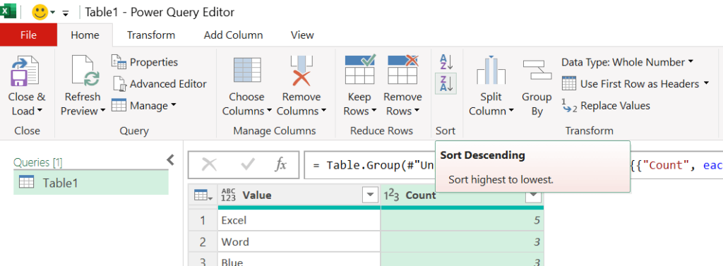
The Text and Numeric values will be arranged in the order of their frequency.
Excel – 5, Red – 4, Grape – 3, etc.,
To remove all text values except the most repeated one,
click on the split button called Keep Rows > Keep Top Rows
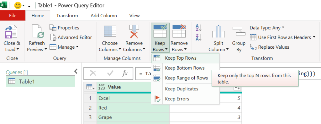
Keep Top Rows dialog will be activated. If you want only the most repeated value, type 1 into the input box for ‘Number of rows’.
For the top two values, I have used 2.

Click OK and we have the Top 2 Most Repeated Values and their count.
Excel – 5 and Red – 4
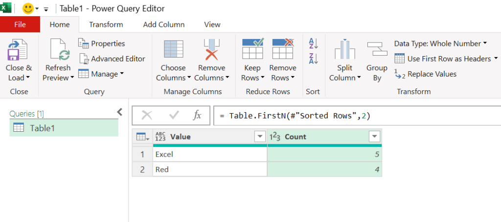
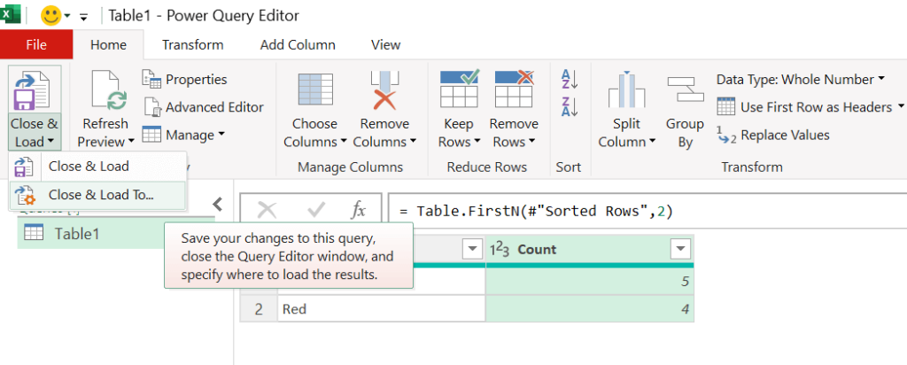
To load this data into the Excel Worksheet,
click on the split button called Close & Load > Close & Load To…
Import Data dialog is activated.
Select Existing worksheet > specify the cell where you want to insert the output from the Power Query Editor
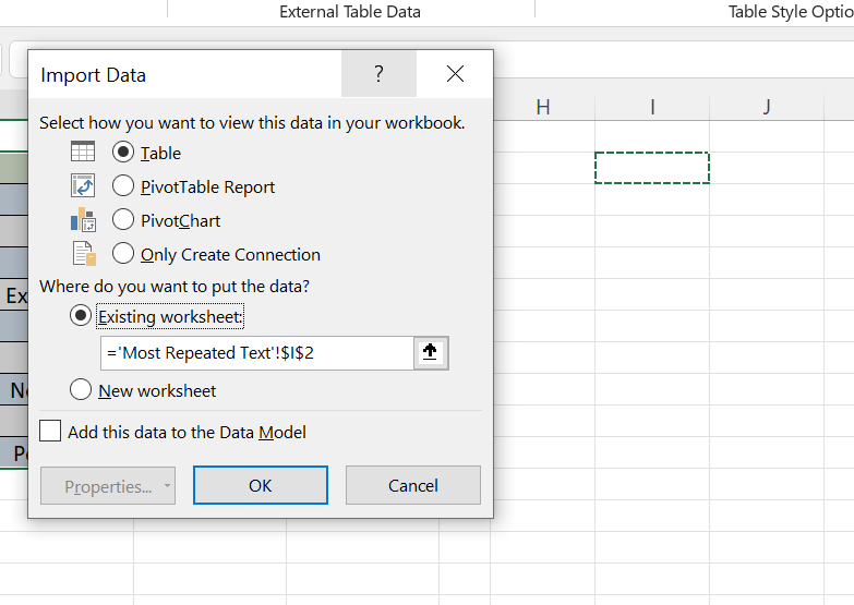
Click OK and we have a new table with the most repeated Text values in the data set.
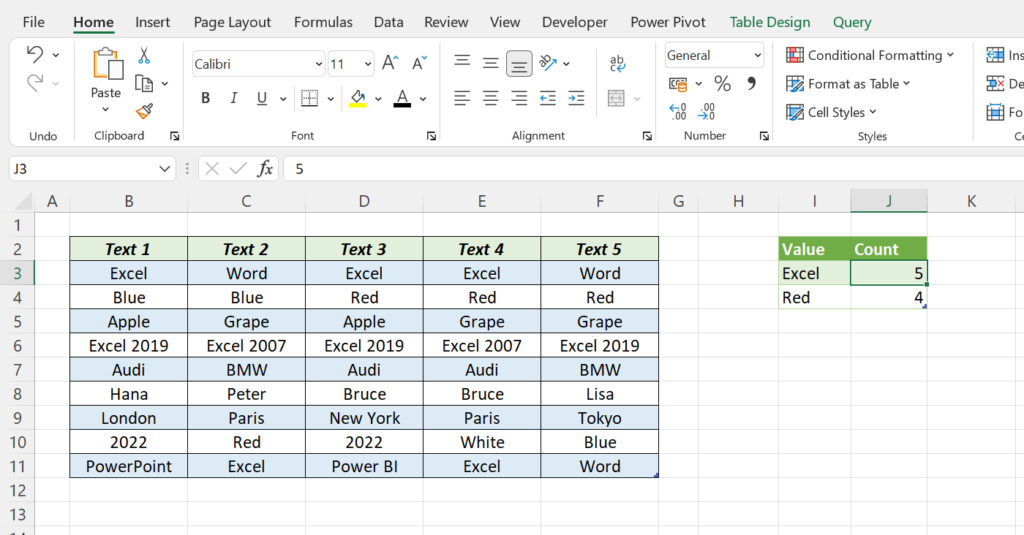
To check the dynamic nature of this method, add few values to the source table and refresh the output table.
