Data in one or more cells can be sent to multiple rows on the basis of delimiters (Comma, Space, etc.) using Power Query in Excel.
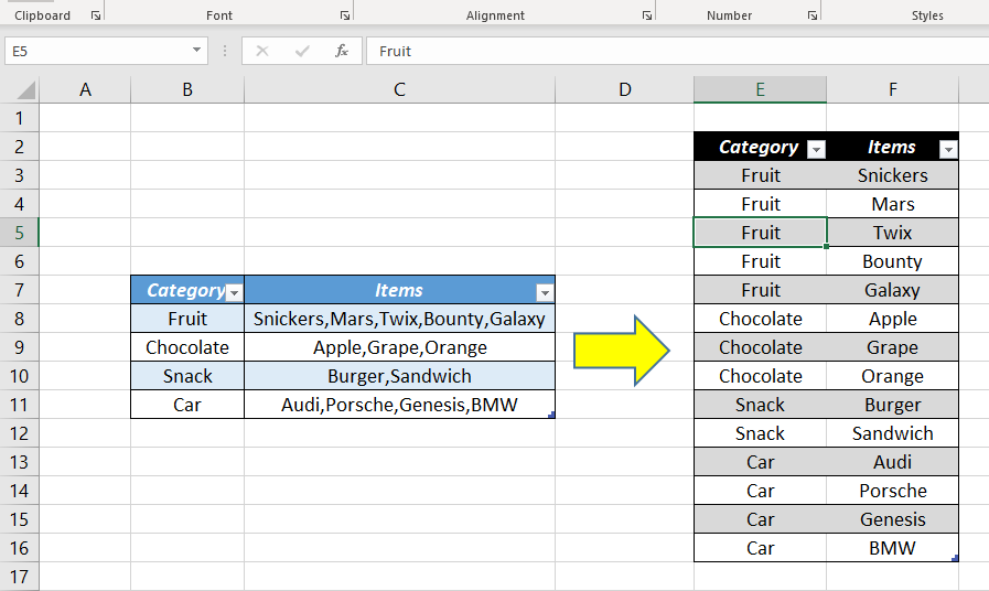
See the example below. Data in the cells C3:C6, which are separated with commas, are exported into the cells E3:F16.
I have used Power Query for this purpose and the procedure I followed is explained below.
Suppose you have a table like the one shown below. Categories are listed in the first column and all Items fall in each category are separated by a comma and listed against the corresponding category name.
To normalize this data, Go to Data Tab in Excel ribbon and Click on From Table/Range
Create Table dialog is activated. Click OK to convert the selected data into an Excel Table.
Power Query Editor is activated and source data is loaded in the editor.
Click on the small down arrow at the bottom of the Split Column button to see a list of available options. By Delimiter, By the number of characters and a few more options are listed here. To split the content of the cells on the basis of comma (,), select the column containing the Items and Click on By Delimiter.
In the Dialog for Split Column by Delimiter, Select Comma from the drop-Ddwn menu and Click OK
Items that were separated with the comma in each cell are now in separate columns.
Select the first column and Click on Unpivot Columns in the Transform Tab
From the drop-down menu of Unpivot Columns, select Unpivot Other Columns.
Now the data is Normalized or columns are Unpivoted. Items that were separated by a comma are now in different rows.
Here the column called Attribute is not necessary and I will remove that column. Right-click on the column and select Remove Other Columns.
Now we have the output which we are looking for and to load this data into the source sheet, Click on Close and Load To
In the Dialog for Import Data, specify the location where you want to place the output table and Click OK.
Here I will use the cell E2 of the same sheet.
The text data that were separated with commas are now in multiple rows of our worksheet. The advantage of Power Query is that you just need to refresh the query for the addition of new data and the table will update for that change.
I will add a new record to the source table.
Energy Drink – Monster, Red Bull, Rockstar Zero
To update the Output table, click on the Refresh button in the Data tab.
Newly added data i.e. the names of different energy drinks (Monster, Red Bull and Rockstar Zero) are appended to the output table.