There are different methods to UnPivot Data in Excel. You can use PivotTable and PivotChart Wizard, Power Query or VBA for this task.
How to UnPivot or Reverse Pivot / Normalize data using Power Query in Excel is explained in this post.
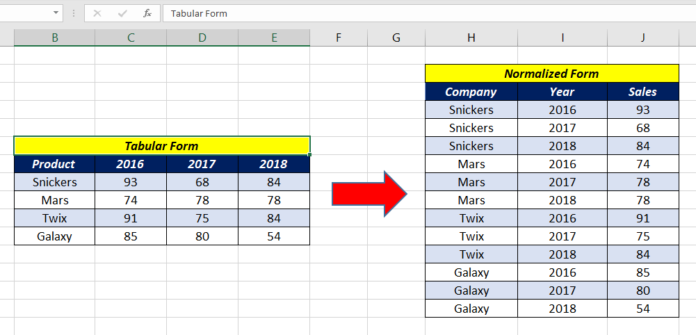
Suppose you have a report like the table shown below.
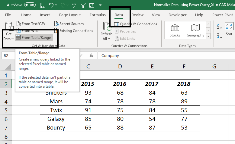
To UnPivot this data using Power Query, we have to convert this data into an Excel Table.
For that, Go to the Data tab of Excel Ribbon > Click on From Table/Range in the Get and Transform data group.
Create Table dialog will be activated.
Click OK and the data range will be converted into an Excel Table, and the Power Query Editor will be activated.
Select all columns except the first column and click on Transform Tab
Click on Unpivot Columns.
Now we have the UnPivotted data or Normalized data
To load this data into the Excel sheet, Go to Home Tab of Power Query Editor, Click on Close and Load.
The following is the Normalized form of Data the Report which we started with.
The advantage of using Power Query is that you just need to Refresh the query for the addition or deletion of data and the table will update for the same.
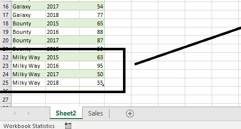
Let me show you what I mean by that. I will add a new line of data to the source table (Milkyway, 63, 95,50 and 55).
To update the table containing Normalized data, Click on Refresh in the Data Tab of Excel Ribbon.
You can see that 4 new rows are added to the bottom of the table.
Following is the video explaining this method in Detail