XLOOKUP is the modern replacement for VLOOKUP. It finds an exact match by default, looks left as well as right, keeps working when columns are inserted, and handles “not found” without IFERROR. If everyone who opens your file has Excel 2021 or Microsoft 365, use XLOOKUP. Here are 8 reasons why, with examples.
Table of Contents
XLOOKUP vs VLOOKUP at a glance
| VLOOKUP | XLOOKUP | INDEX + MATCH | |
|---|---|---|---|
| Default match | Approximate (risky) | Exact | Exact with 0 |
| Look to the left | No | Yes | Yes |
| Inserting a column | Can break it | Safe | Safe |
| Built-in “not found” | No, needs IFERROR | Yes | No |
| Return several columns | One per formula | Yes, spills | One per formula |
| Last match | No | Yes | Complex |
| Next larger value | No, next smaller only | Yes | Yes |
| Horizontal lookup | Needs HLOOKUP | Yes | Yes |
| Works in Excel 2019 and earlier | Yes | No | Yes |
Compare the syntax:
=VLOOKUP(lookup_value, table_array, col_index_num, [range_lookup])=XLOOKUP(lookup_value, lookup_array, return_array, [if_not_found], [match_mode], [search_mode])VLOOKUP needs a table and a column number. XLOOKUP needs the column to search and the column to return, which is simpler to read and harder to get wrong.
1. XLOOKUP finds an exact match by default
VLOOKUP uses an approximate match unless you add FALSE as the fourth argument. Forget it, and VLOOKUP can quietly return a wrong value. XLOOKUP is exact with just three arguments:
=XLOOKUP(B3,F4:F10,H4:H10)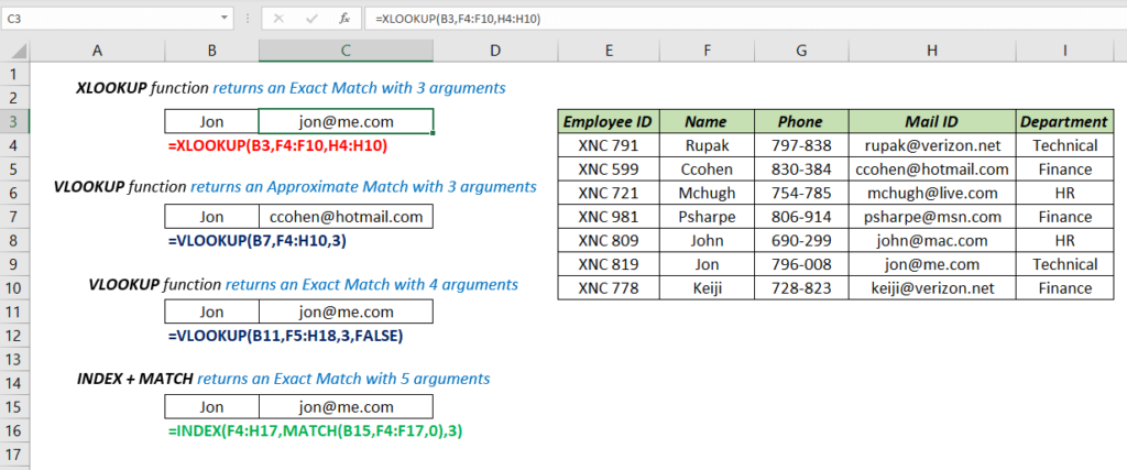
VLOOKUP needs =VLOOKUP(B11,F5:H18,3,FALSE) for the same result, and INDEX + MATCH needs two functions.
2. XLOOKUP can look to the left
VLOOKUP can only return values from columns to the right of the one it searches. XLOOKUP doesn’t care where the return column is. This finds the name from an email address in a column further right:

With VLOOKUP, you’d have to move columns around or use a CHOOSE trick. INDEX + MATCH can also look left, but XLOOKUP does it with one function.
3. Inserting a column doesn’t break XLOOKUP
VLOOKUP’s column number is typed into the formula. Insert a column in the middle of the table, and col_index_num of 3 now points at the wrong column, without any error message.
| Before inserting a column | After inserting a column | |
|---|---|---|
| VLOOKUP | Returns Phone (column 3) | Returns the new column instead: wrong |
| XLOOKUP | Returns Phone | Still returns Phone: the reference moves with the column |
This is the most common cause of silent VLOOKUP errors in shared workbooks.
4. A custom message when nothing is found
VLOOKUP returns #N/A when there’s no match, so it’s usually wrapped in IFERROR. XLOOKUP has a fourth argument for it:
=XLOOKUP(B3,F4:F10,H4:H10,"Employee not found")
Unlike IFERROR, it only replaces “not found”. Real errors, such as a typo in the formula, still show up so you can fix them.
5. Return several columns with one formula
Give XLOOKUP a multi-column return range and it spills all of them. One formula returns the name, phone, email and department for an employee ID:
=XLOOKUP(B12,B3:B9,C3:F9)
With VLOOKUP, you’d need one formula per column, each with a different column number.
6. Find the last match, not just the first
VLOOKUP always stops at the first match. Set XLOOKUP’s sixth argument, search_mode, to -1 to search from the bottom up:
=XLOOKUP(G3,C3:C10,D3:D10,,,-1)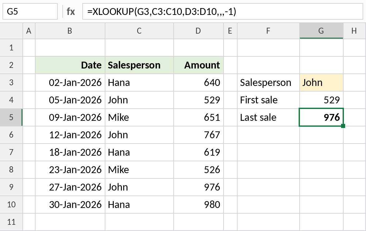
Without the sixth argument, XLOOKUP returns John’s first sale, 529. With -1, it returns his latest, 976. The data doesn’t need to be sorted.

| search_mode | Searches |
|---|---|
1 or omitted |
First to last |
-1 |
Last to first |
2 |
Binary search on data sorted A to Z (fast on huge lists) |
-2 |
Binary search on data sorted Z to A |
7. Return the next larger value
For bands and slabs, VLOOKUP’s approximate match can only return the next smaller value. XLOOKUP’s fifth argument, match_mode, can go either way. Here, a tax table lists the upper limit of each slab, so the formula needs the next larger limit:
=XLOOKUP(C8,$G$4:$G$9,$H$4:$H$9,,1)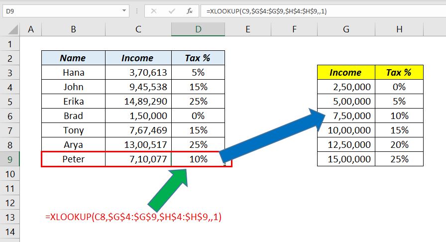
An income of 7,10,077 isn’t in the table, so XLOOKUP uses the next larger limit, 7,50,000, and returns 10%. The lookup column doesn’t need to be sorted either, unlike VLOOKUP’s approximate match.
| match_mode | Finds |
|---|---|
0 or omitted |
Exact match |
-1 |
Exact match or the next smaller value |
1 |
Exact match or the next larger value |
2 |
Wildcard match with * and ? |
8. One function for vertical and horizontal lookups
VLOOKUP only works down columns, so tables laid out across need HLOOKUP. XLOOKUP works both ways. Point it at a row instead of a column:
=XLOOKUP("Mar",C2:H2,C3:H3)That returns the March value from a table with months across the top.
When VLOOKUP is still the right choice
- Older Excel versions. XLOOKUP shows
#NAME?in Excel 2019, 2016 and earlier. If you share files with people using them, stick with VLOOKUP or INDEX + MATCH. - Existing workbooks that work. There’s no need to rewrite every VLOOKUP. Use XLOOKUP for new formulas.
- Google Sheets supports both, so either is fine there.
Frequently asked questions
Is XLOOKUP available in Excel 2019?
No. XLOOKUP is in Excel 2021, Excel 2024, Microsoft 365 and Excel for the web. In Excel 2019 and earlier, use VLOOKUP or INDEX + MATCH.
Is XLOOKUP better than INDEX + MATCH?
They can do most of the same things, but XLOOKUP needs one function instead of two, has a built-in “not found” argument, and can search from the bottom up. INDEX + MATCH is still useful when you need compatibility with older versions.
Is XLOOKUP slower than VLOOKUP?
Not noticeably for normal workbooks. For very large sorted lists, XLOOKUP’s binary search modes (2 and -2) are faster than either.
Can XLOOKUP replace HLOOKUP?
Yes. XLOOKUP works on rows and columns, so it replaces both VLOOKUP and HLOOKUP.