To look up a value that matches two or more conditions, such as the sales for North *and* Pen, join the conditions together. Here are three ways: XLOOKUP for Excel 365, INDEX and MATCH for every version, and a helper column for plain VLOOKUP.
Excel 365: XLOOKUP with joined criteria
North appears three times and Pen twice, but only one row has both. Join the two criteria, and join the two columns, so XLOOKUP looks for “NorthPen”:
=XLOOKUP(G2&G3,B3:B10&C3:C10,D3:D10)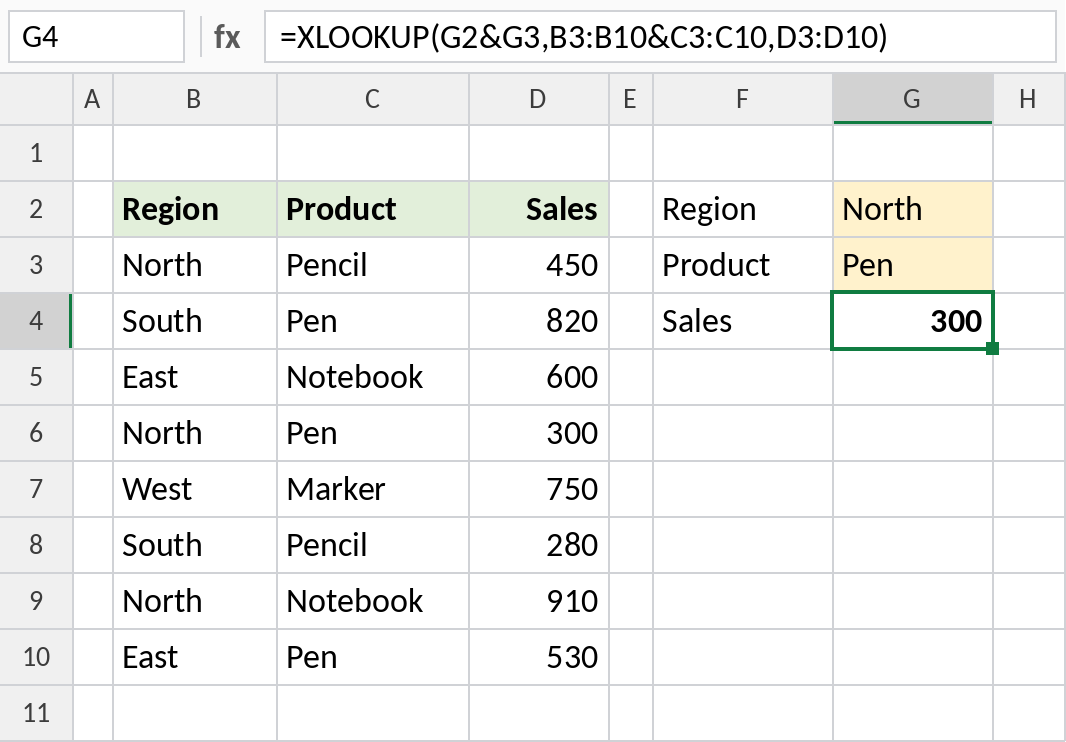
The only row with North and Pen is row 6, so the result is 300. A plain lookup on North alone would have returned 450, the first North row.
How the formula works
G2&G3joins the criteria into NorthPen.B3:B10&C3:C10joins the two columns row by row: NorthPencil, SouthPen, EastNotebook, NorthPen…- XLOOKUP finds NorthPen in that joined list and returns the matching value from D3:D10.
Any version: INDEX and MATCH
Each test returns TRUE or FALSE for every row. Multiplying them gives 1 only where both are TRUE, and MATCH finds that 1:
=INDEX(D3:D10,MATCH(1,(B3:B10=G2)*(C3:C10=G3),0))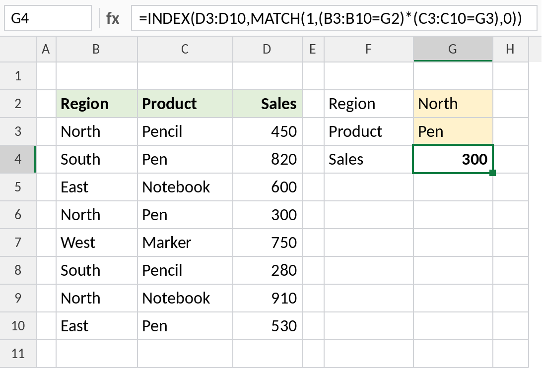
The result is the same, 300. In Excel 2019 and earlier, confirm the formula with Ctrl+Shift+Enter.
Plain VLOOKUP: add a helper column
VLOOKUP searches only one column, so build one: column B joins region and product with a dash. Then look up the joined value:
=VLOOKUP(H2&"-"&H3,B3:E10,4,FALSE)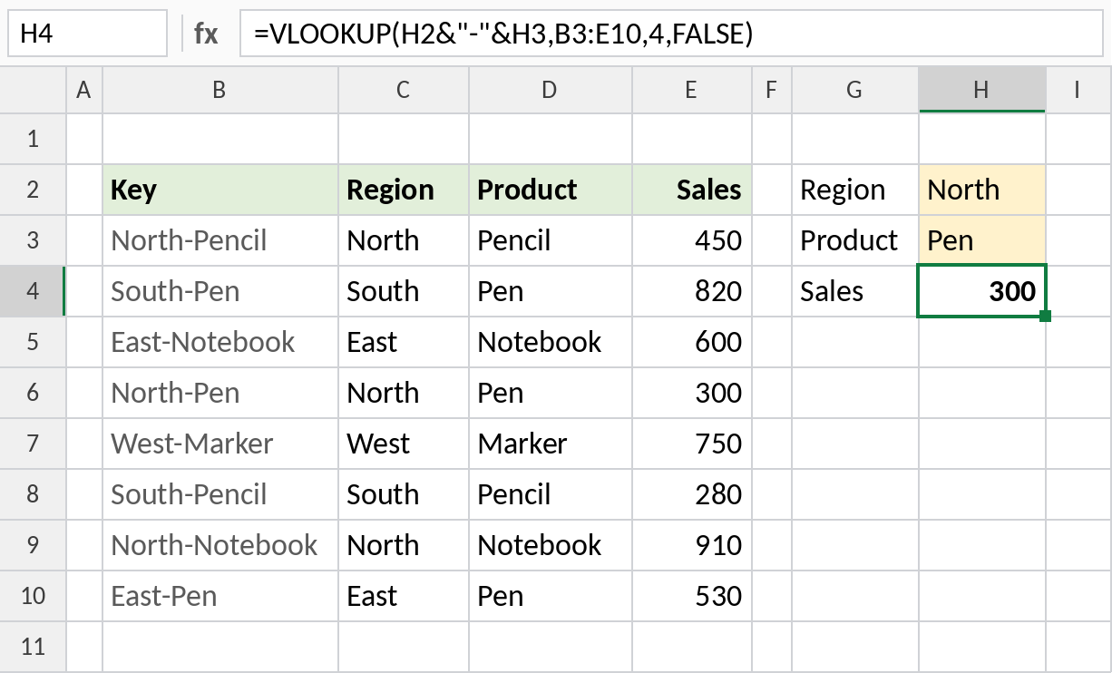
VLOOKUP finds North-Pen in the helper column and returns column 4, Sales: 300. The dash stops mix-ups such as “AB”+”C” matching “A”+”BC”.
Which method to use
| Method | Works in | Needs |
|---|---|---|
| XLOOKUP with & | Excel 2021, 365 | Nothing extra |
| INDEX + MATCH | All versions | Ctrl+Shift+Enter in 2019 and earlier |
| VLOOKUP + helper column | All versions | An extra column |
| SUMIFS | All versions | Numbers only, and each combination must be unique |
For three or more criteria, keep joining: G2&G3&G4 and B3:B10&C3:C10&D3:D10.
Notes
- If no row matches every criterion, the formula returns
#N/A. Use XLOOKUP’s fourth argument or IFERROR for a message. - If several rows match, these formulas return the first one. To return all of them, use FILTER.
- Joined criteria are text, so numbers stored as text and as numbers still match.
Common errors
| Problem | Cause | Fix |
|---|---|---|
#N/A |
No row matches all criteria, or extra spaces | Check spellings; use TRIM |
#VALUE! in old Excel |
INDEX/MATCH entered without Ctrl+Shift+Enter | Confirm as an array formula |
| Wrong match | Joined values overlap | Join with a separator such as a dash |
Practice file
All three methods, with the helper column already set up.