Slicers are floating filters associated with PivotTable, PivotChart and official Tables in Excel. Apart from filtering data, Slicers also provide the current filtering status.
In this blog post, we will see how to add Slicers for PivotTables and Excel Tables. We will also cover how to ‘Connect a Slicer to two or more PivotTables.’
Table of Contents
Add Slicer for an Excel Table
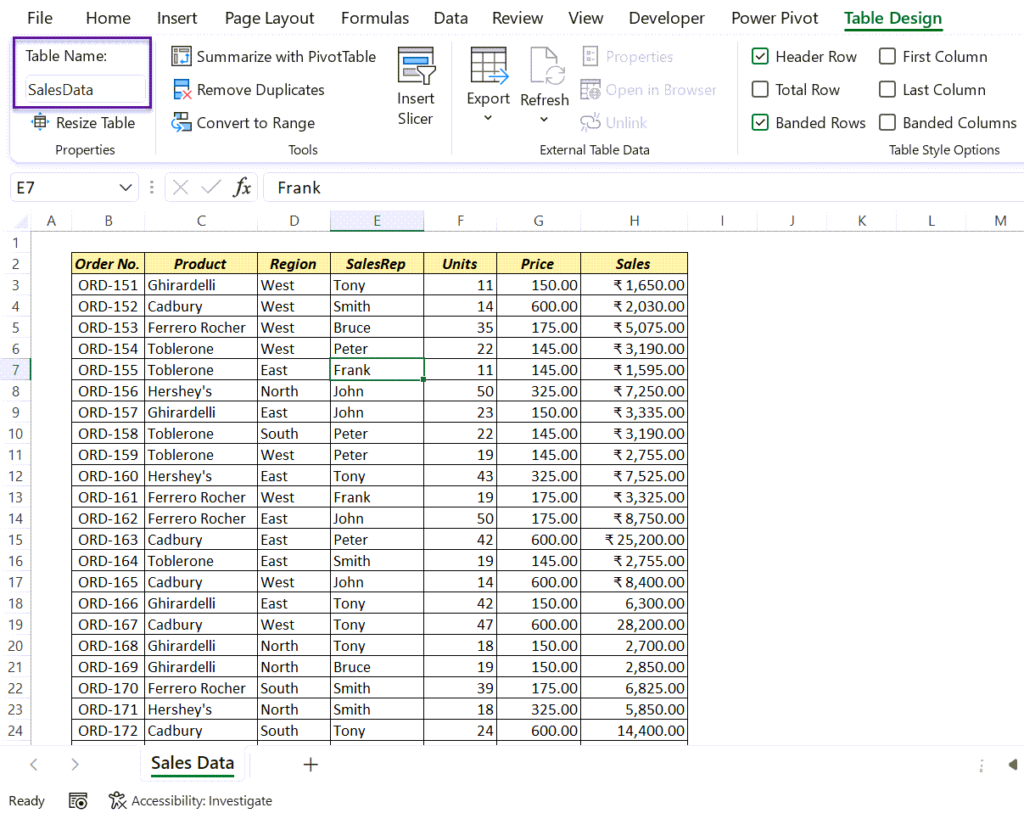
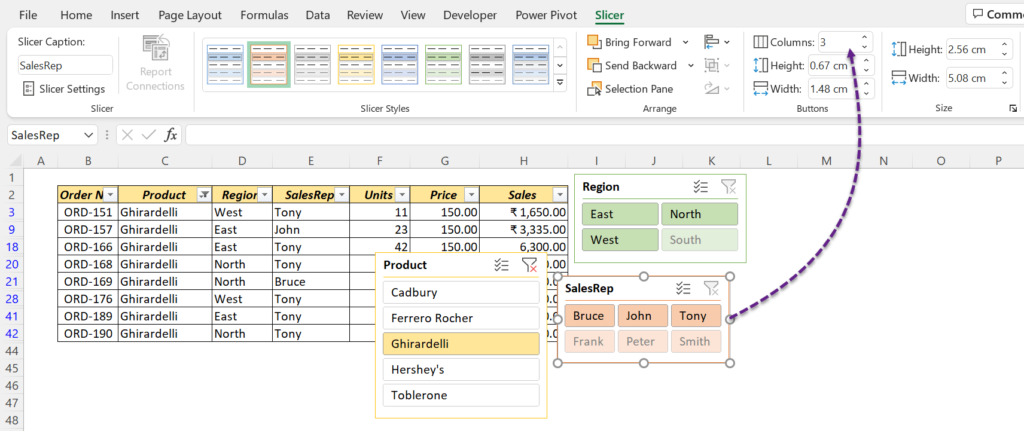
Following is an Excel Table called SalesData which contains the sales records of a company that deals with Chocolates like Ghirardelli, Cadbury, Ferrero Rocher, Toblerone in the East, West, South and North Regions of Cochin city.
The table also contains the details of the Sales executives responsible for the sales.
Suppose, I want to filter the above sales report and go through the sales figures of different Products in West and North Regions of Cochin.
Of course we can use the Filter tool in Excel to filter this data. But the easiest way to do this is using Slicers.
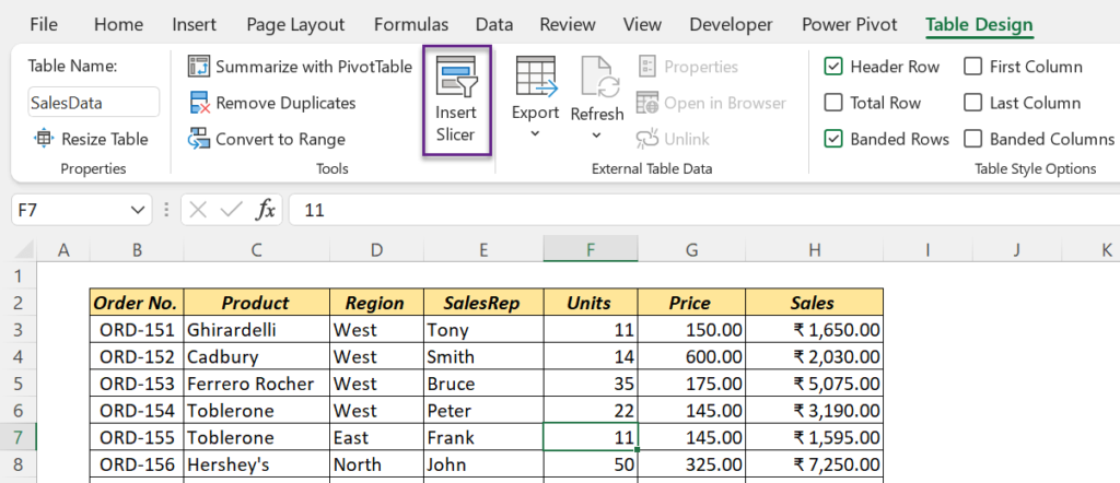
To add Slicers for the table called SalesData,
select the table > go to the Table Design tab > Click on Insert Slicer
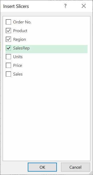
A dialog called Insert Slicers is activated, which contains the list of columns in the selected table.
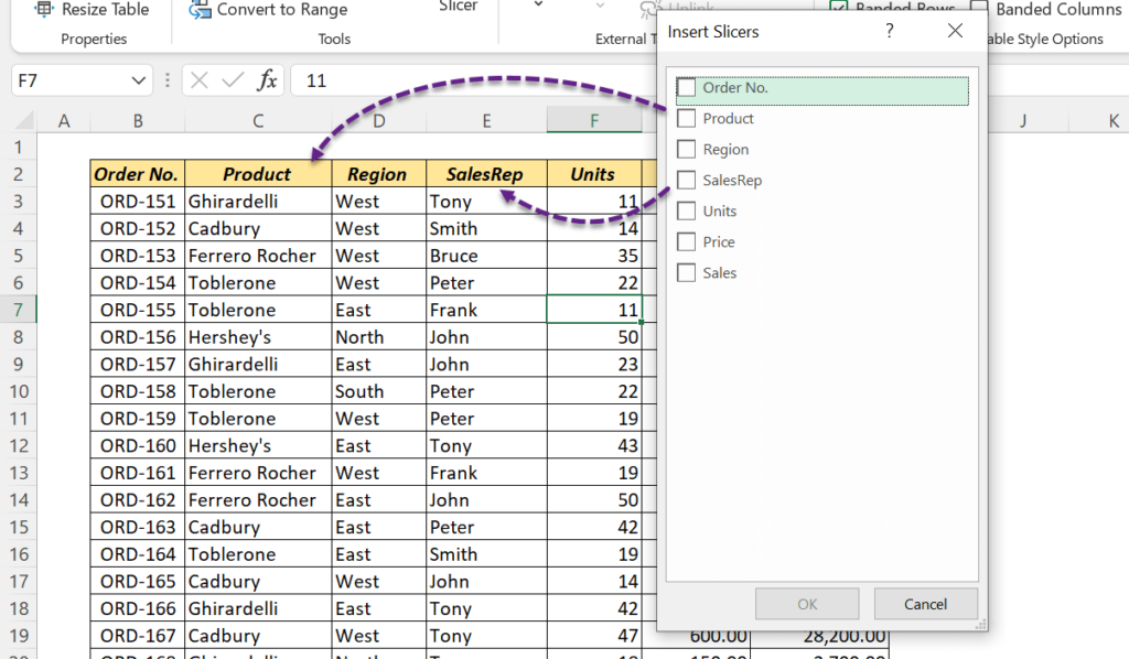
In this case we need the Slicers for ‘Product’, ‘Region’ and ‘SalesRep’.
Mark the corresponding checkboxes and click on OK.
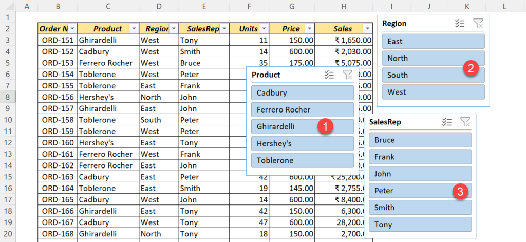
3 Slicers are inserted. 1. Product, 2. Region and 3. SalesRep.
Now, let’s see how to use these Slicers.
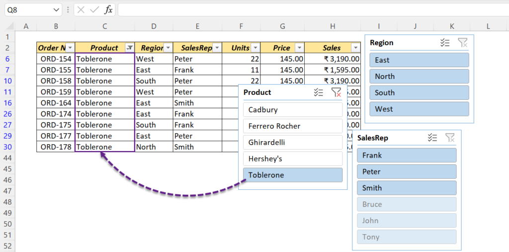
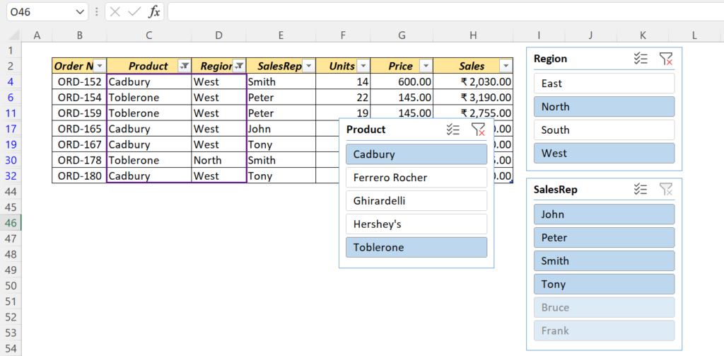
In case, you want to see only the records related to Toblerone, click on the button called Toblerone in the Slicer called Product.
For the records related to Toblerone and Cadbury, holding the Ctrl key, click on the button for Cadbury.
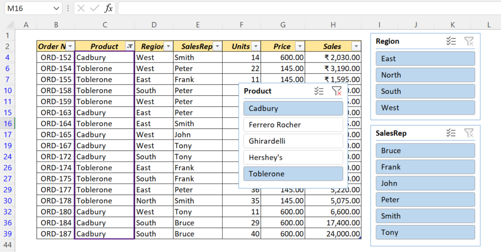
You may have noticed that all buttons in the corresponding Slicer other than the selected ones, got faded.
For the sales of Toblerone in the West and North regions of Cochin, click on the buttons called West and North arranged in the slicer called Region.
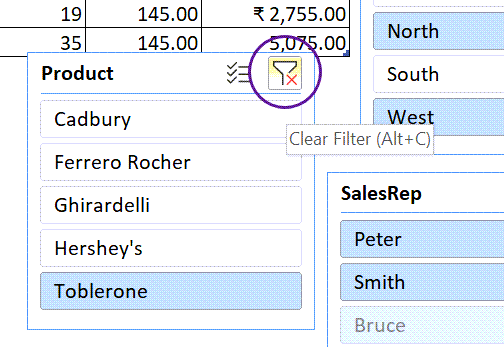
To remove the filter applied using a Slicer, click on the button called Clear Filter in the top right corner of the corresponding slicer.
To remove a Slicer, right-click on the Slicer and select ‘Remove Slicer Name’
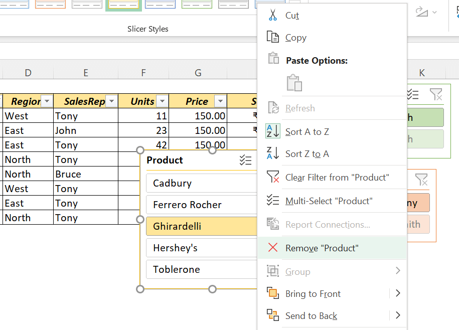
You can also get rid of Slicers using the Delete button on the keyboard.
Modifying the Slicer
There are a few ‘Predefined Slicer Styles’ available in Excel that can be used to change the appearance of a Slicer.
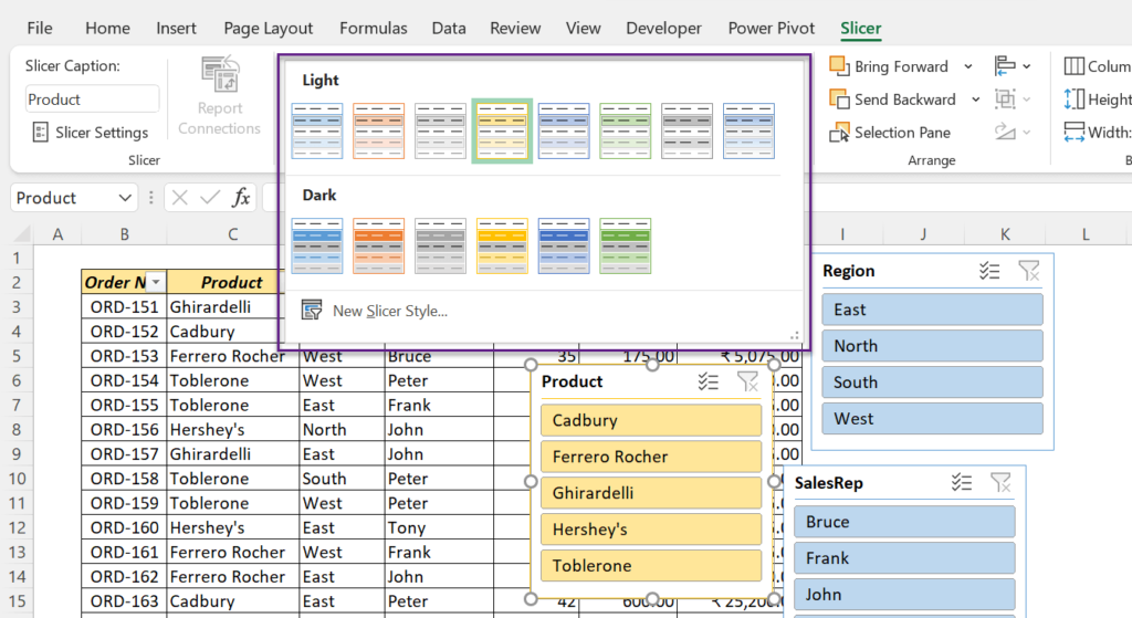
We can also create new styles using the New Slicer Style… option.
Height and Size of a Slicer as well as the ‘Buttons’ on them can modified and the buttons on a Slicer can be arranged in multiple columns.
Add Slicer for a PivotTable
Adding Slicers for a PivotTable is quite similar to the procedure we followed for an Excel Table.
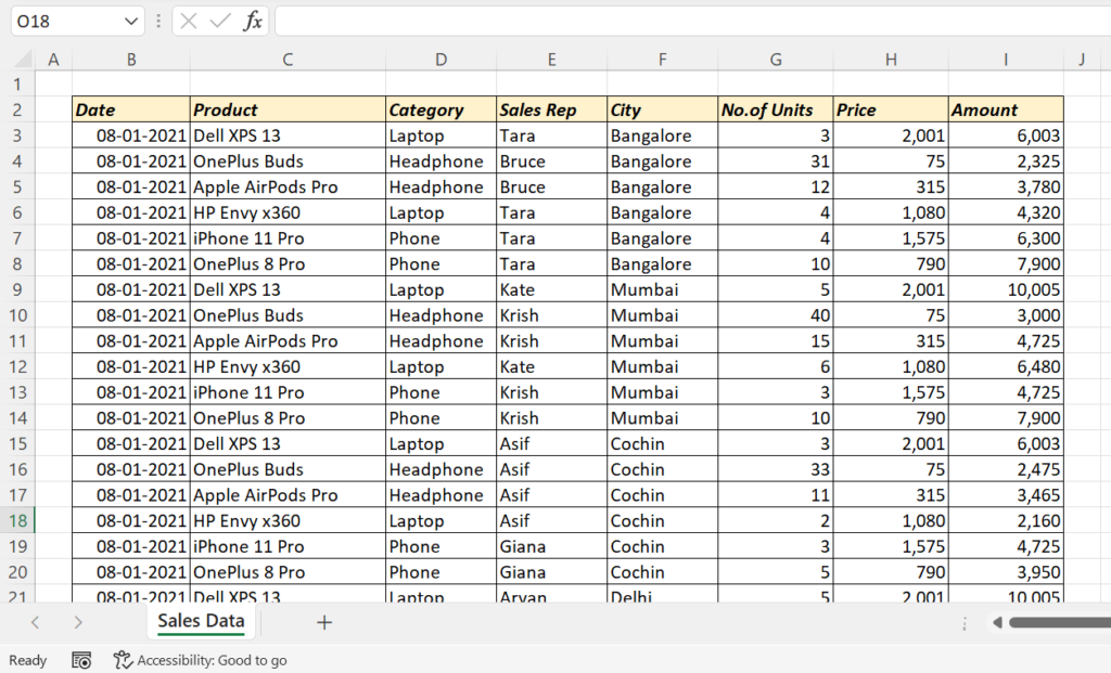
Following is the the Sales records of a company that deals with the Head phones, Cell phones and Laptops in different cities of India.
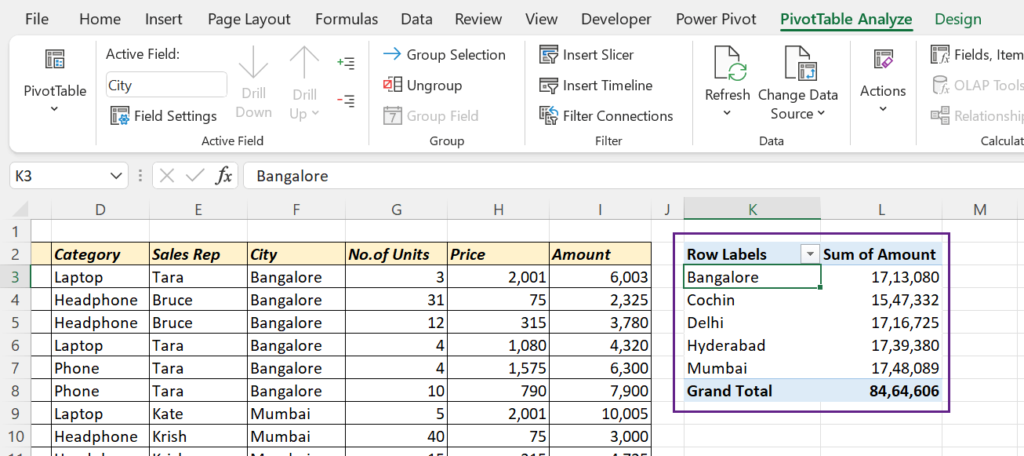
And here is a Pivot Table created from the above data to find the sales happened in each city.
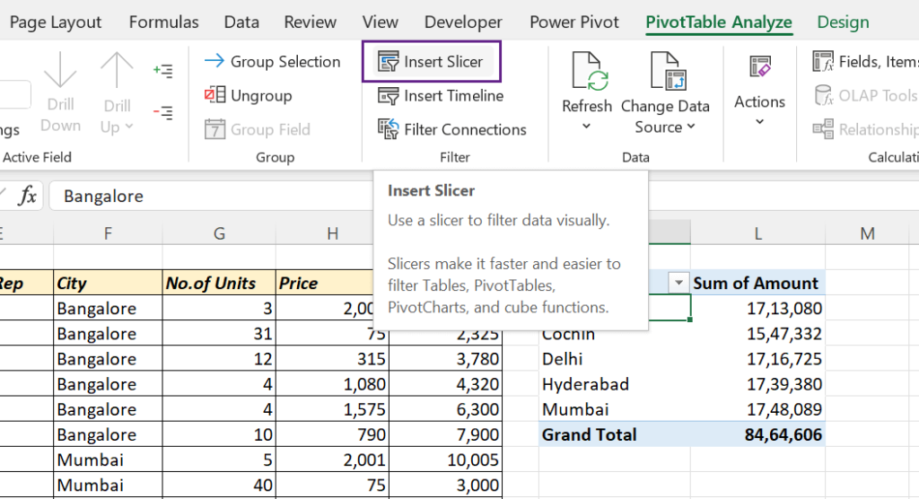
To add Slicers which will help us to filter this Pivot Table,
Click on the PivotTable > go to the PivotTable Analyze tab > click on Insert Slicer
The dialog called Insert Slicer is activated. Mark the required checkboxes and Click OK.
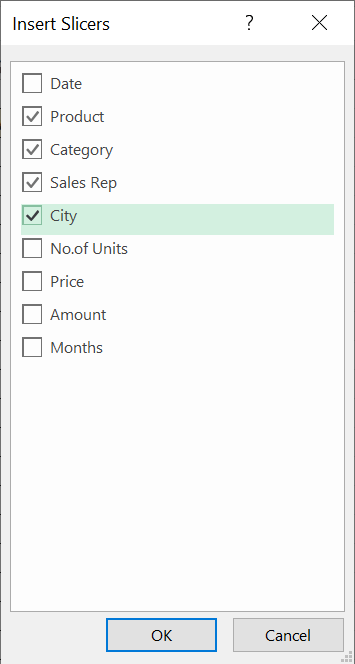
As I selected the Slicers for Sales Rep, Category, Product and City, 4 Slicers are inserted.
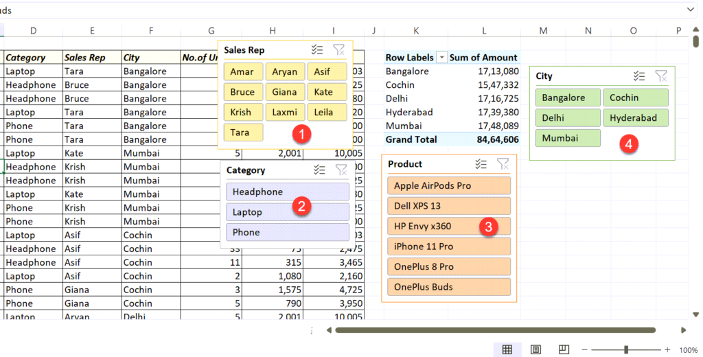
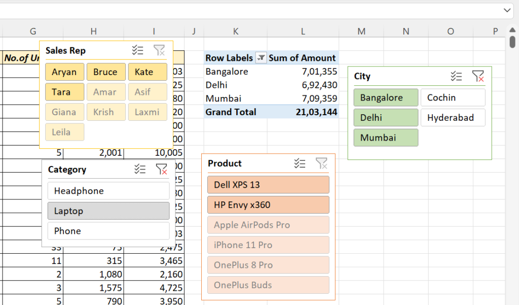
In case, we need the Sale figures for Laptop in the cities Bangalore, Delhi and Mumbai,
click on the buttons for Bangalore, Delhi and Mumbai on the Slicer called ‘City’ and the button for Laptop on the Slicer called ‘Category’.
Connect a Slicer to multiple Pivot Tables
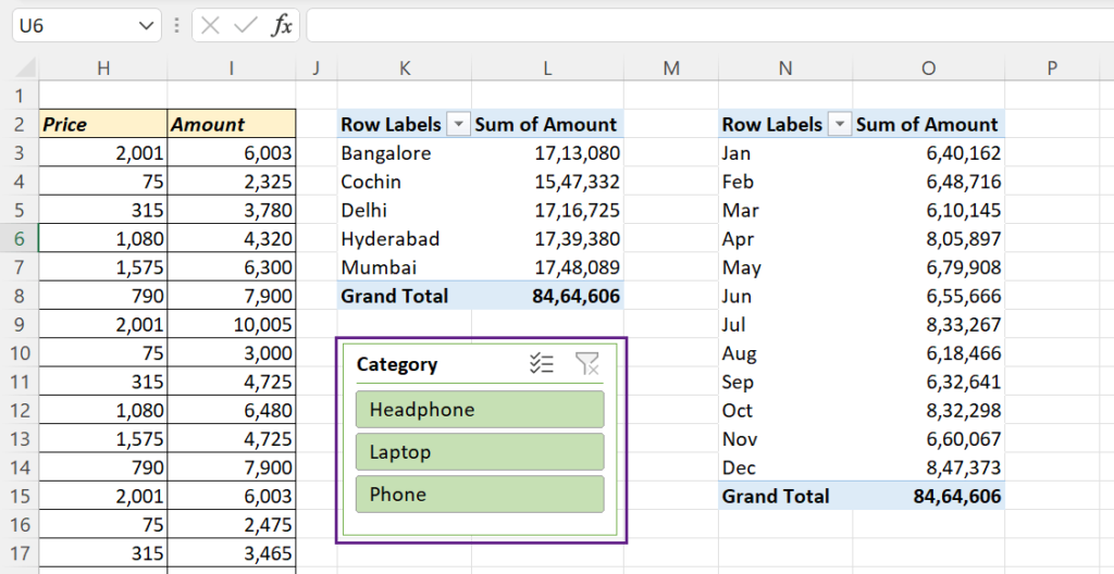
A single Slicer can be used to filter data in multiple Pivot Tables.
Let’s see, How to connect the Slicer called Category to both the PivotTables show below.
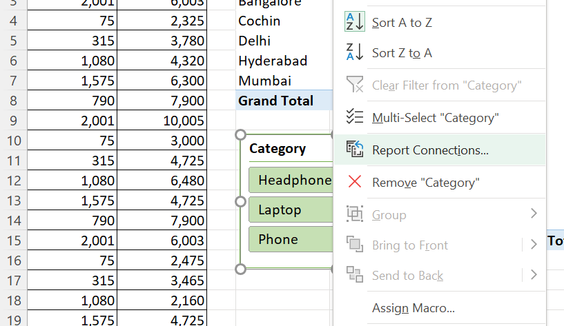
Right-click on the Slicer called Category > select Report Connections…
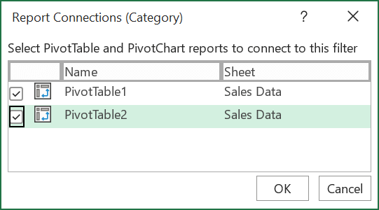
In the dialog called Report Connections (Slicer Name), we will have the list of the available Pivot Tables.
Mark the checkbox for the second PivotTable and click OK
Now when we use the Slicer called Category, both PivotTable1 and PivotTable2 will update accordingly.