This blog post is about combining the NOW function with the Conditional Formatting feature in Excel to highlight a cell or cells corresponding to Current Time.
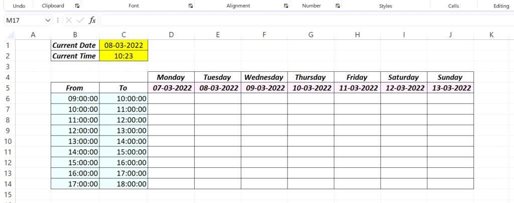
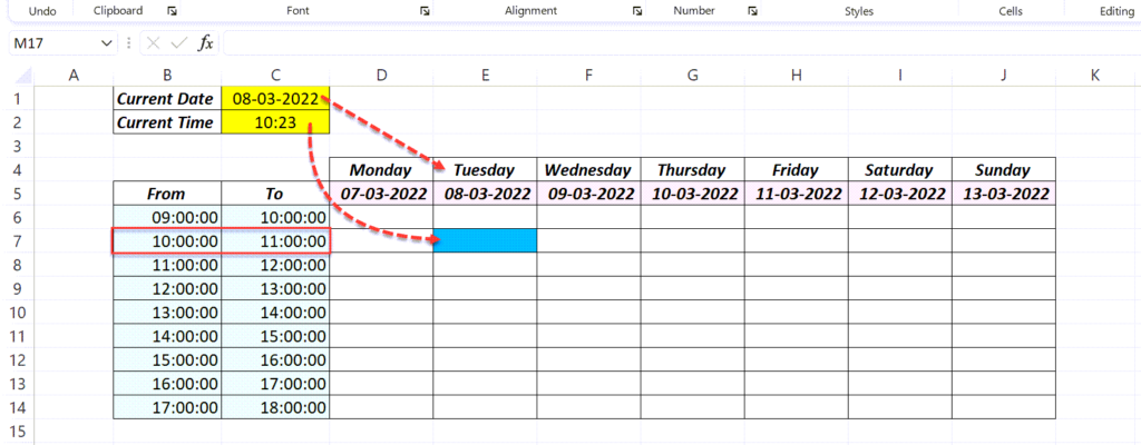
The following is a very common spreadsheet template used at working environments for recording manhours. Let’s see how to spot the cell corresponding to 10:23 A.M (Current Time) on 08/03/2022 (Current Date).
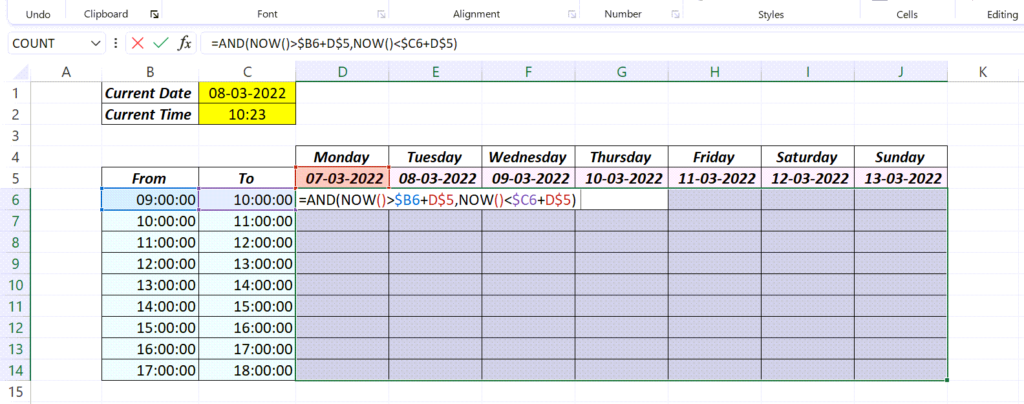
All blank cells in the template are selected and the following formula is typed in.
=AND(NOW()>$B8+D$5,NOW()<$C8+D$5)
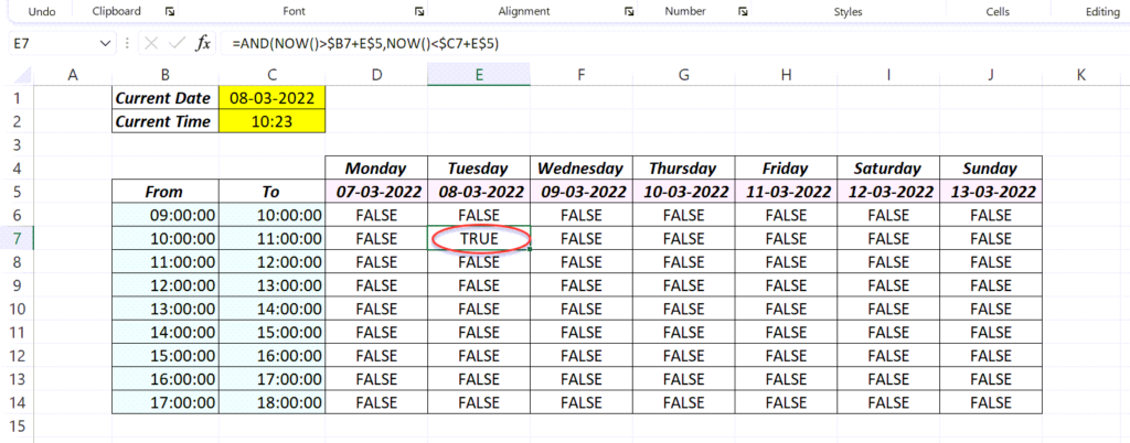
All cells except E7 have FALSE in it.
The TRUE in the cell E7 means, the Current Time falls in between 10:00 and 11:00 on 08/03/2022.
Here the TRUE and FALSE values are generated for your understanding. Let’s see how to use the same formula with Conditional Formatting to highlight the cell corresponding to current Time.
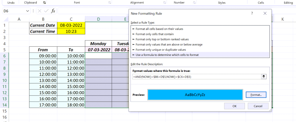
Clear the formula that generated TRUE, FALSE values > Once again select the cells > In the Home tab of the Excel ribbon > Conditional Formatting > New Rule…
In the New Formatting Rule dialog, select a ‘Use a formula to determine which cells to format’ and type in the formula which we used to generate TRUE and FALSE values.
=AND(NOW()>$B8+D$5,NOW()<$C8+D$5)
After entering the formula, use the Format button to define the formatting in which you want to highlight the cell. Here I have selected Blue color for this purpose.
When I took the following screenshot, it was 10:23 A.M on 08/03/2022 and you can see the cell E7 corresponding that Date and Time is highlighted in blue.
If I check this worksheet an hour later, the next cell E8 will be highlighted in blue color.