A hyperlink lets you jump from a summary sheet straight to the detail behind a number. Use the HYPERLINK function, Insert Link (Ctrl + K), or the little-known right-drag trick.
The example
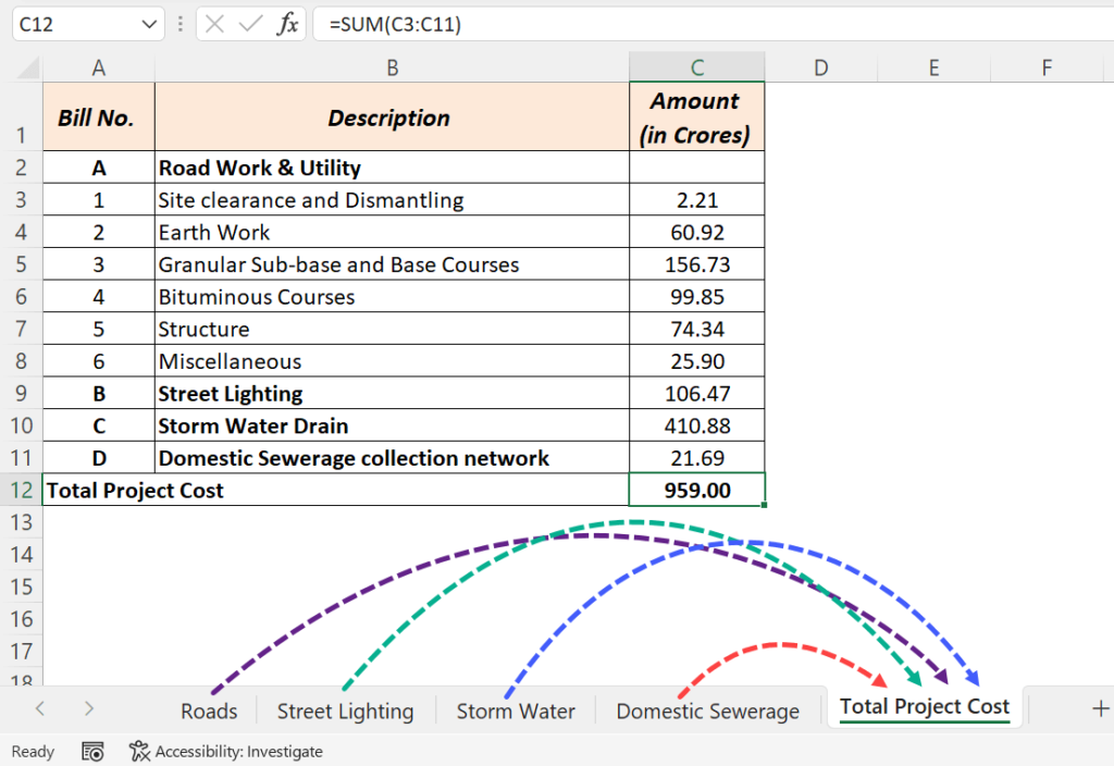
A highway project’s cost summary pulls each total from its own sheet: Roads, Street Lighting, Storm Water and Domestic Sewerage. Each amount should open the sheet it came from.
1. HYPERLINK function
HYPERLINK takes a link location and the text to show. Put # before the sheet name to mean this workbook:
=HYPERLINK("#'Roads'!F4",Roads!F4)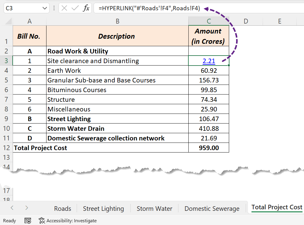
The second argument, Roads!F4, shows the amount itself, so the cell still displays the number. Sheet names with spaces need single quotes:
=HYPERLINK("#'Street Lighting'!G217",'Street Lighting'!G217)
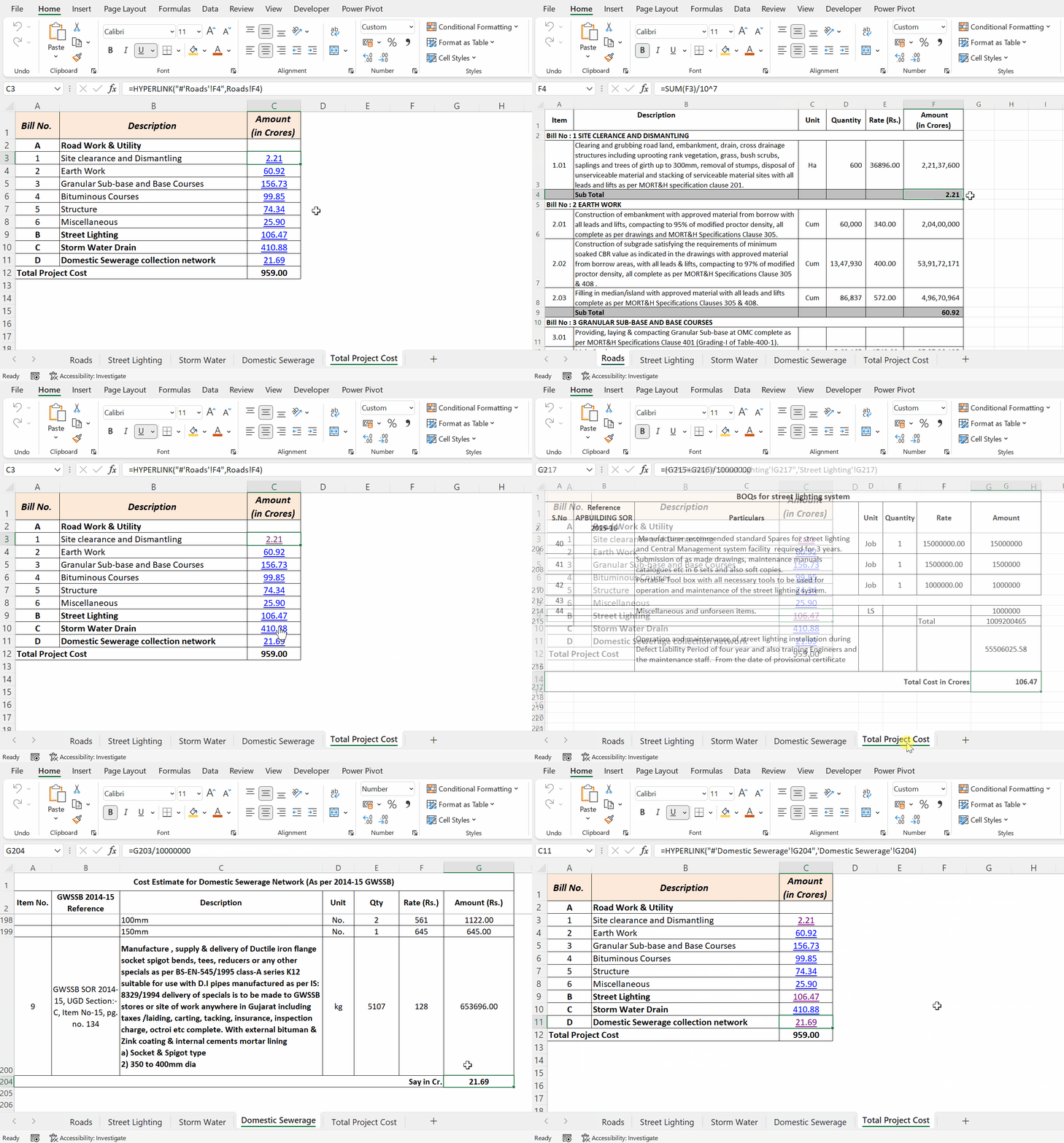
2. Insert Link (Ctrl + K)
- Right-click the cell and choose Link, or press Ctrl + K.
- Click Place in This Document.
- Choose the sheet, type the cell (such as F4) and click OK.


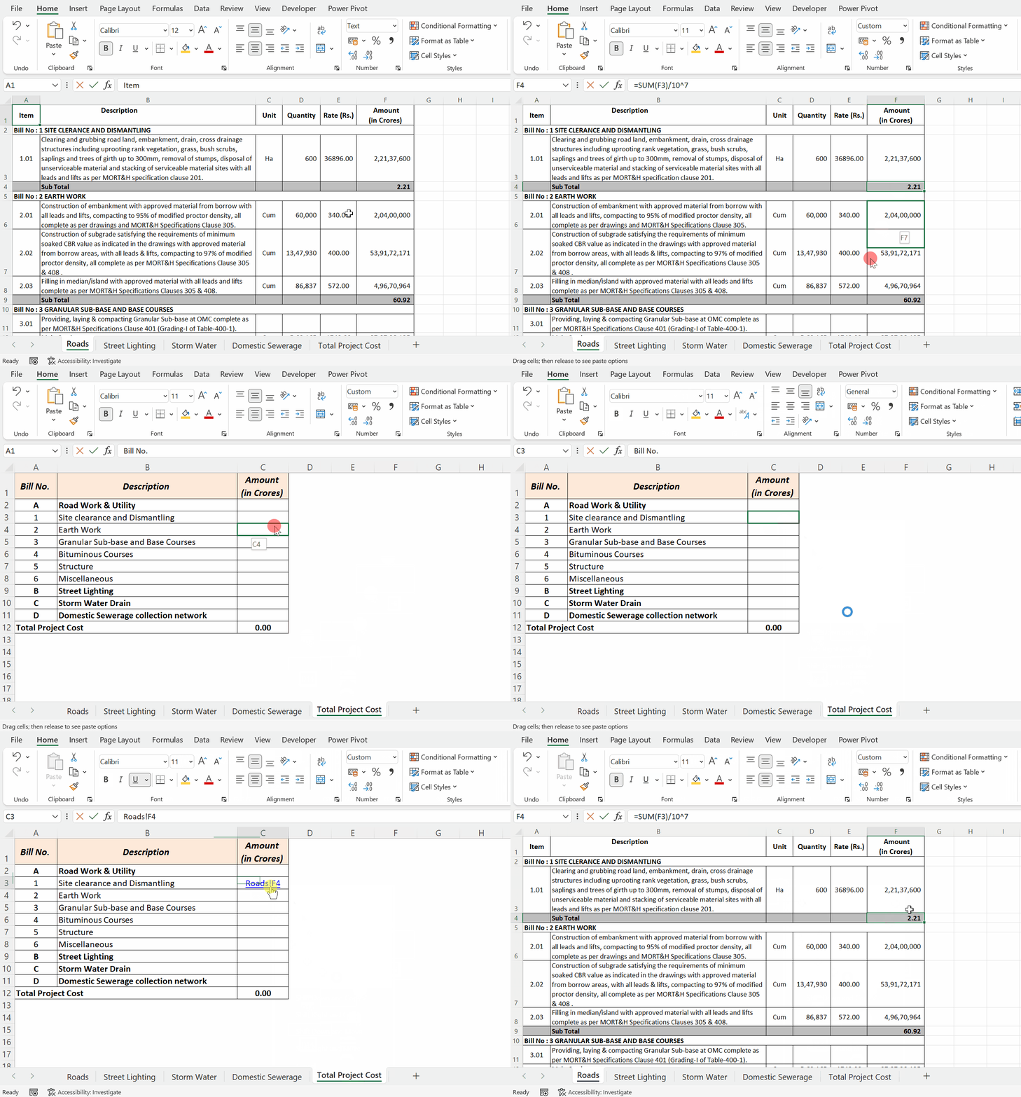
3. Right-drag with Alt (fastest)
- Select the target cell and point at its border until the cursor becomes a four-way arrow.
- Hold the right mouse button and Alt, and drag onto the sheet tab where you want the link.
- Drop on the cell and choose Create Hyperlink Here.


On the same sheet you don’t need Alt.
Links that survive renaming a sheet
All three methods store the sheet name as text, so renaming Roads to Road Works breaks the link. To avoid that, give the target cell a name (type RoadsTotal in the Name Box) and link to the name:
=HYPERLINK("#RoadsTotal",Roads!F4)Names follow the cell when sheets are renamed or rows are inserted.
Things to know
- To select a linked cell without following it, click and hold until the pointer changes, or select it with the arrow keys.
- For a clickable list of every sheet, use the table of contents macro.
- HYPERLINK also opens web pages and files:
=HYPERLINK("https://xlncad.com","XL n CAD").