This tutorial is about 7 different methods to Remove Duplicates in Excel.
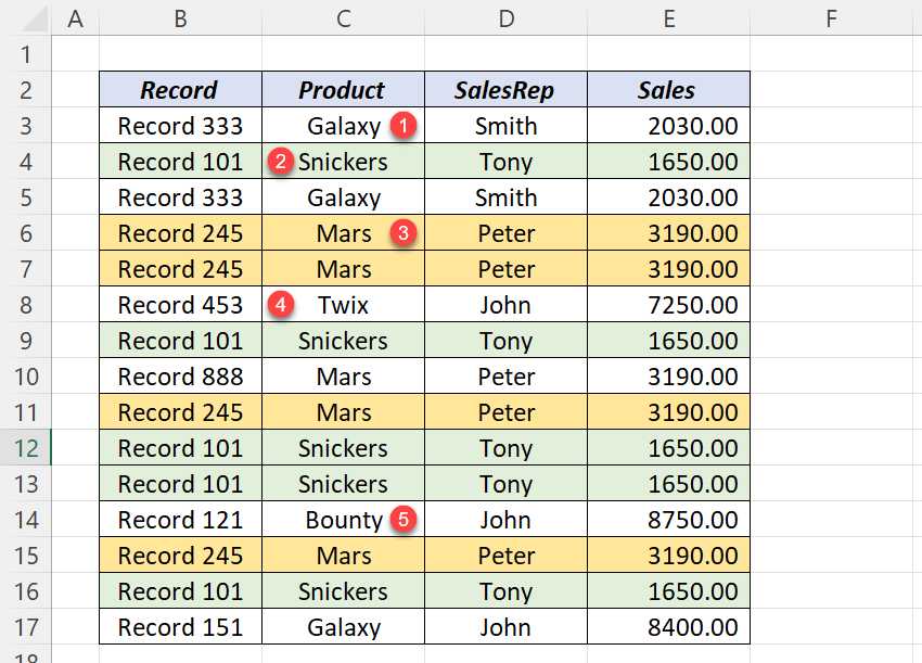
I will be using the following data to explain the different ways to get rid of the records that repeat multiple times.
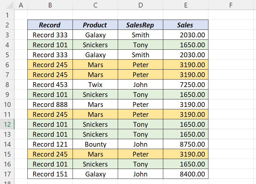
Table of Contents
Remove Duplicates tool in Excel
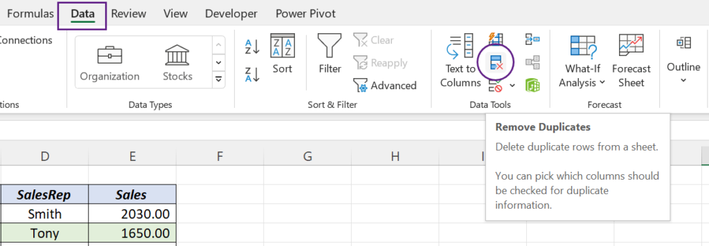
The Remove Duplicates feature in Excel is the most popular tool for removing duplicates and is placed in the Data tab of the Excel ribbon.
To get rid of duplicate records from a dataset,
select the cells containing data > go to the Data tab of the Excel ribbon > click on Remove Duplicates
Remove Duplicates dialog will be activated and all those columns in the selected data set will be listed in this dialog.
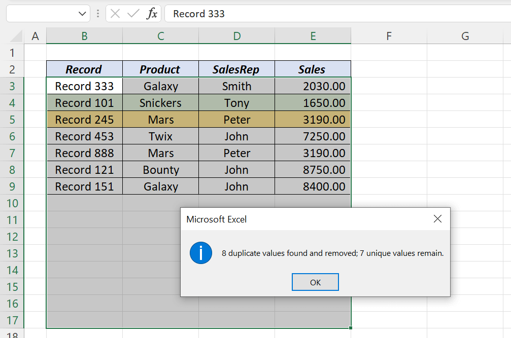
If the dataset has column headers, mark the checkbox against the label, My data has headers.
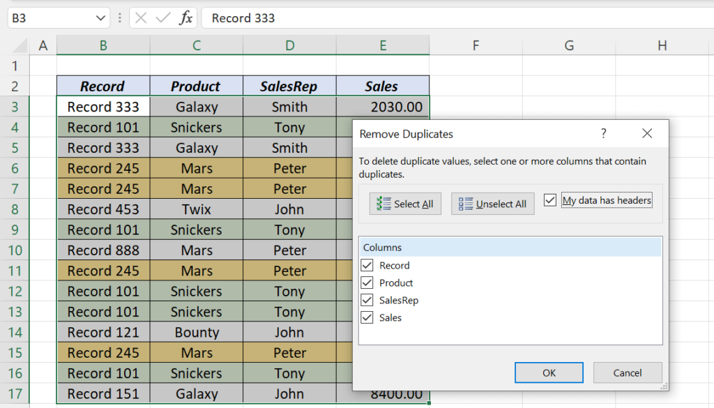
Click OK and we will get a message box about the status of cleaning. In this case, 8 duplicate records were removed and we are left with 7 unique records.
The Remove Duplicates tool can also be used to get rid of duplicates from a specific column or columns.
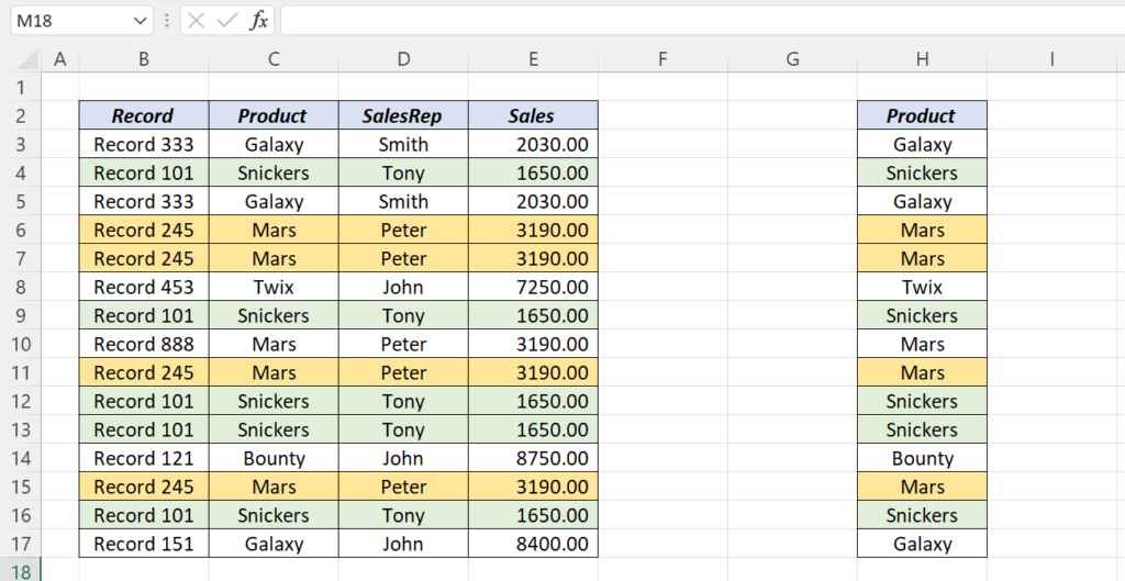
Suppose, I need the list of products from our data set.
It will be better to make a copy of the column called Product so that the source data won’t get affected.
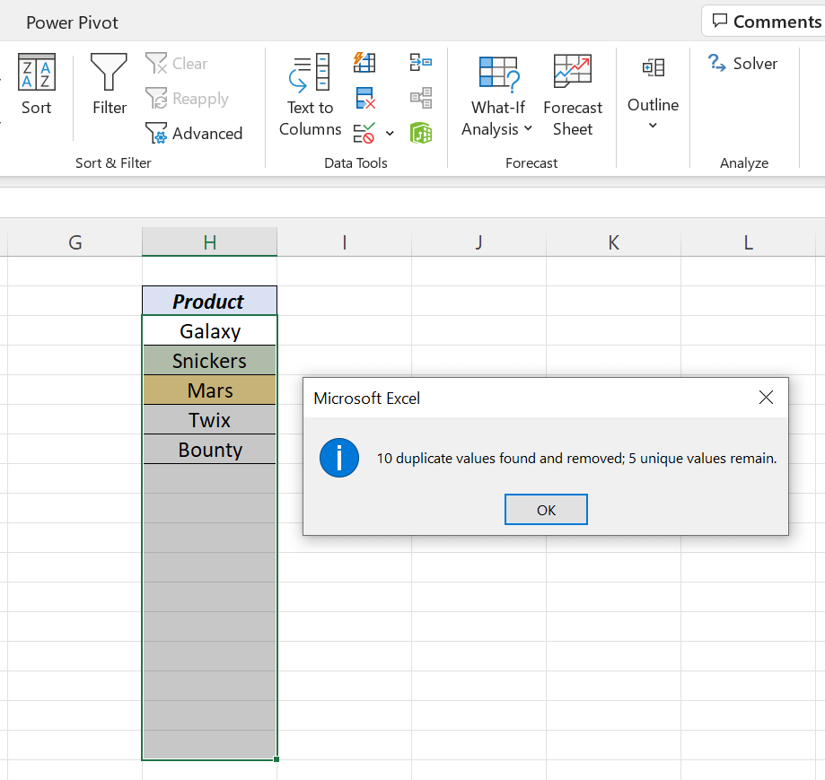
Select the copied column and click on Remove Duplicates.
The Remove Duplicates dialog will be activated and the selected column will be listed in this dialog.
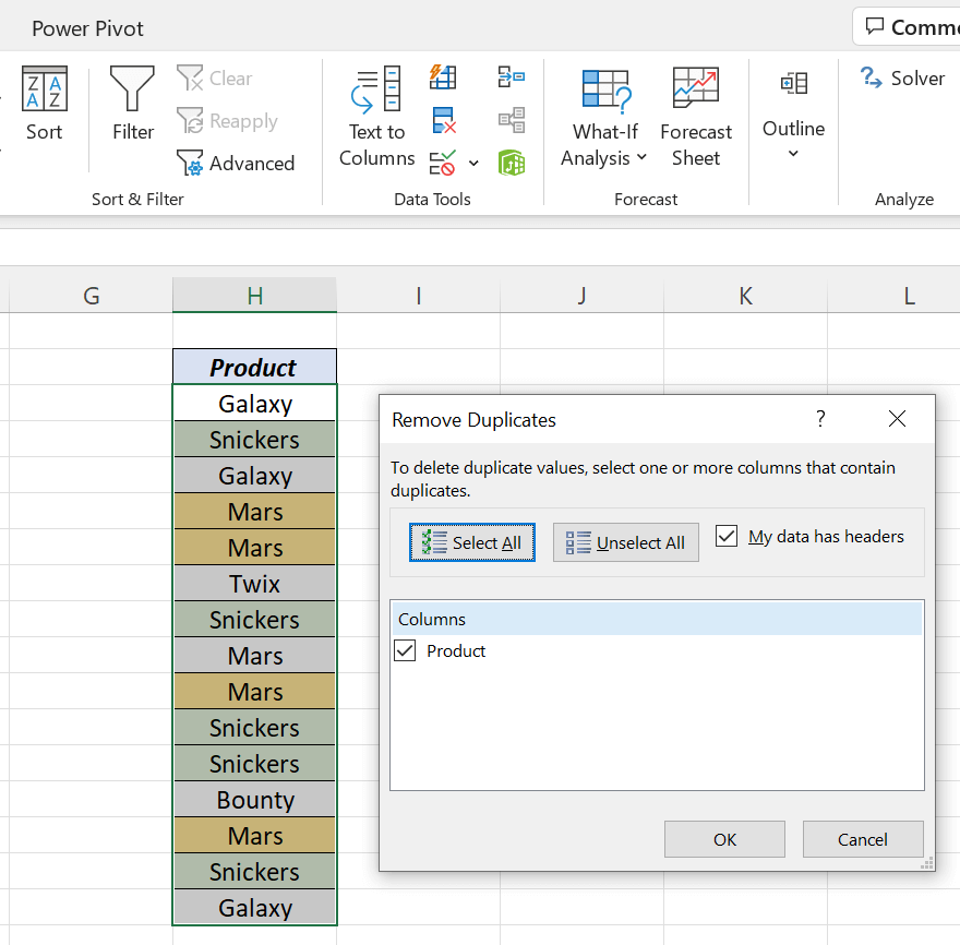
Click OK and we have the list of products.
Advanced Filter to remove duplicates
Unlike the normal Filter tool, the Advanced Filter in Excel helps us to extract records on the basis of the specified conditions. The same can be used to create the unique list of records from a data set.
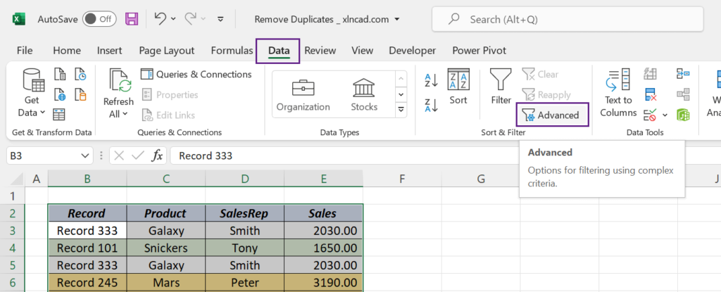
To remove duplicates from a data set,
select the cells containing data > go to the Data tab of the Excel ribbon > Advanced
The Advanced Filter dialog will be activated.
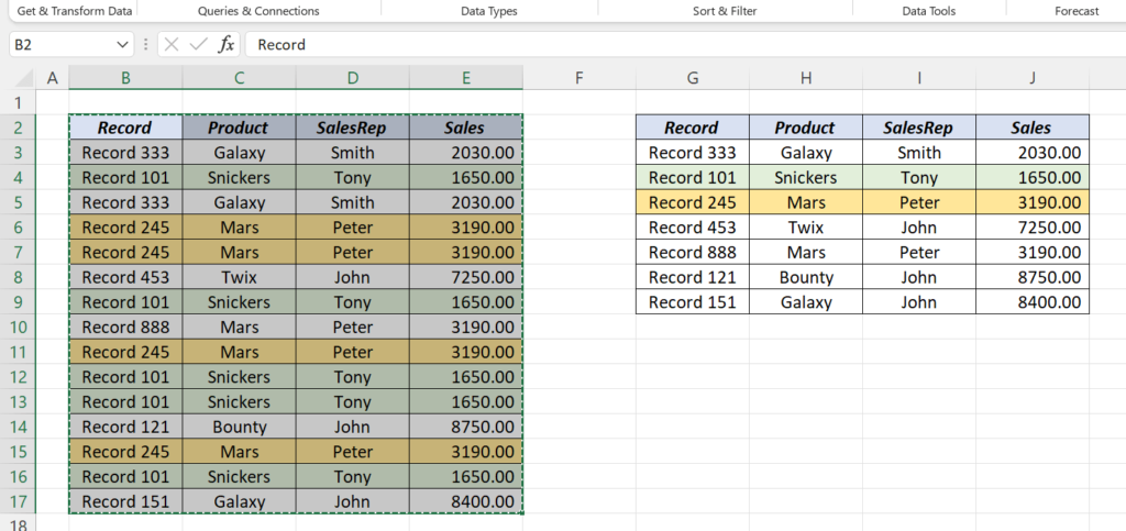
As we have selected the source data just before activating the Advanced Filter, the address of that data range ($B$2:$E$17) is displayed in the input box against the label, List range.
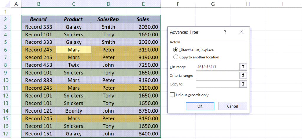
Click on the radio button for Copy to another location
Specify the address of the destination (the cell G2 of the same sheet) in the input box against Copy to:
Click on the up arrow on the right side of this input box for manual selection.
Mark the check box against the label Unique records only.
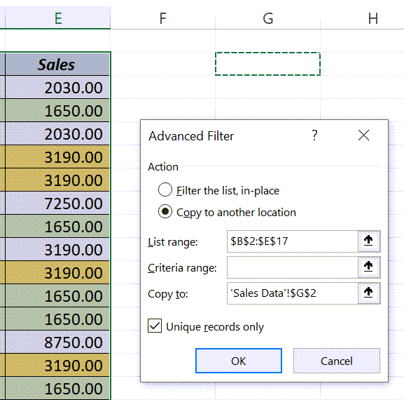
Click OK and the unique records from the selected data set are extracted to the cell G2.
UNIQUE Function to remove duplicates
The UNIQUE function is one of the Dynamic Array Functions in Excel and can be used to create the ‘unique list’ of records from a data set.
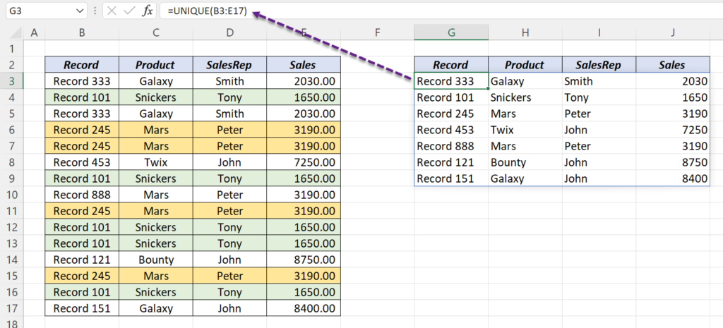
The following formula will return the unique list of records present in the range B3:B17
=UNIQUE(B3:E17)
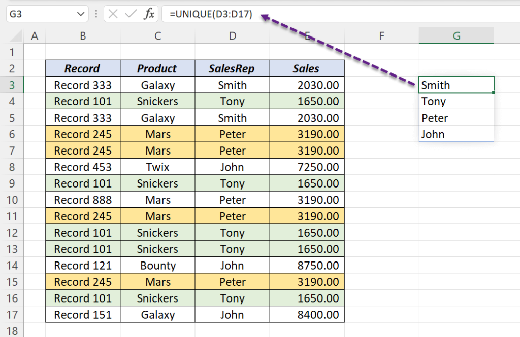
Suppose we need the list of Sales representatives from the same data. Supply the column (D3:D17) containing the name of Sales representatives into the UNIQUE function.
=UNIQUE(D3:D17)
COUNTIF Function to remove duplicates
In this method, we will use the COUNTIF function to spot the duplicates in a dataset.
As we have data in multiple columns, the TEXTJOIN function is to combine the values in each row.
=TEXTJOIN("",,B3:E3)
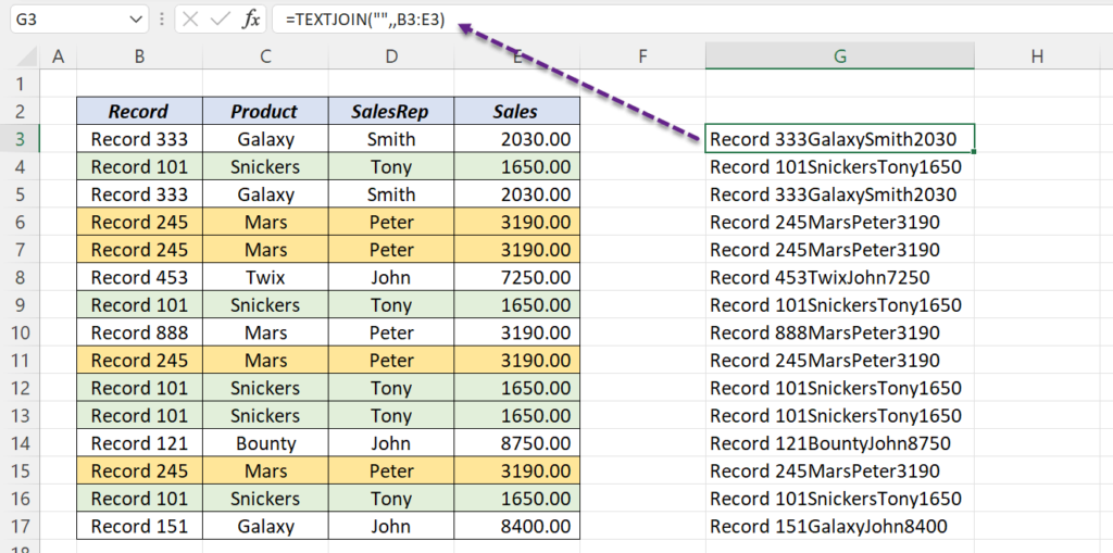
The COUNTIF function is then used to find the records that are repeated more than once.
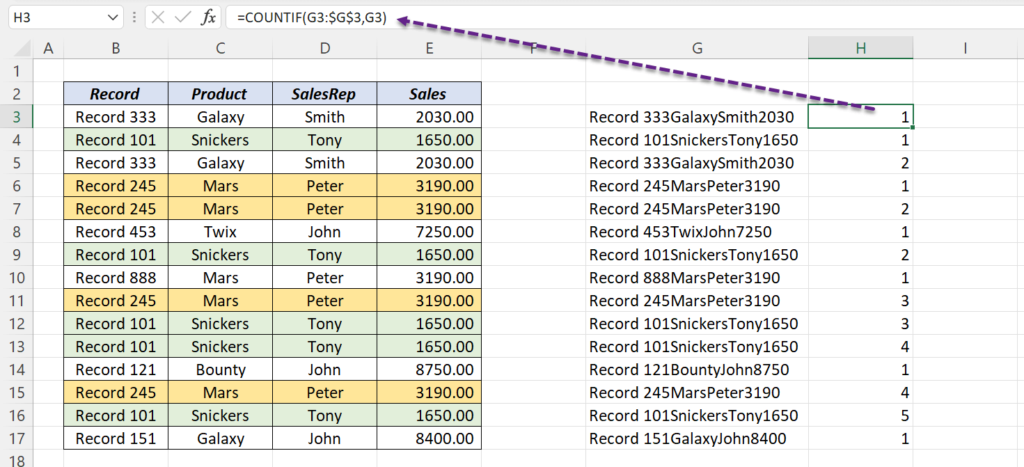
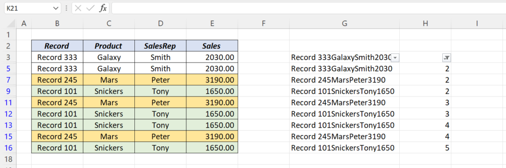
Apply filter for the values greater than 1 and manually delete those rows.
Macro to remove duplicates
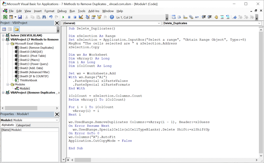
The following macro when executed, will create a unique list of records from the selection and insert it into a new Worksheet.
Sub Delete_Duplicates()
Dim xSelection As Range
Set xSelection = Application.InputBox("Select a range", "Obtain Range Object", Type:=8)
MsgBox "The cells selected are " & xSelection.Address
xSelection.Copy
Dim ws As Worksheet
Dim vArray() As Long
Dim i As Long
Dim iColCount As Long
Set ws = Worksheets.Add
With ws.Range("A1")
.PasteSpecial xlPasteValues
.PasteSpecial xlPasteFormats
End With
iColCount = xSelection.Columns.Count
ReDim vArray(1 To iColCount)
For i = 1 To iColCount
vArray(i) = i
Next i
ws.UsedRange.RemoveDuplicates Columns:=vArray(i - 1), Header:=xlGuess
On Error Resume Next
ws.UsedRange.SpecialCells(xlCellTypeBlanks).Delete Shift:=xlShiftUp
On Error GoTo 0
ws.Columns("A").AutoFit
Application.CutCopyMode = False
End Sub
Paste the above code into the VBA Editor of Excel and execute the Macro called Delete_Duplicates.
Power Query to remove duplicates
To remove the duplicate records from a data set using Power Query,
select the cells containing data > go to the Data tab of the Excel ribbon > click on From Table/Range
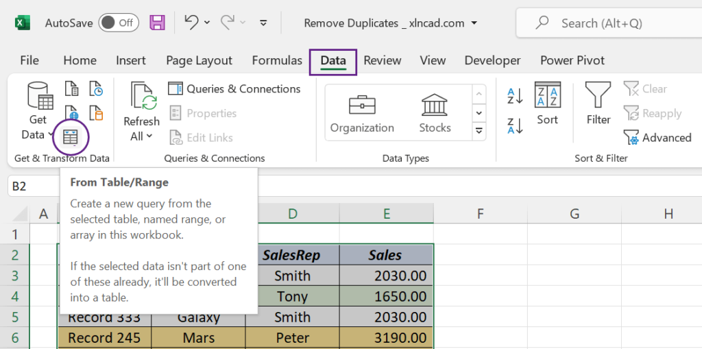
If the selected data range is not an official Excel Table, we will be prompted to convert that data range into an Excel Table.
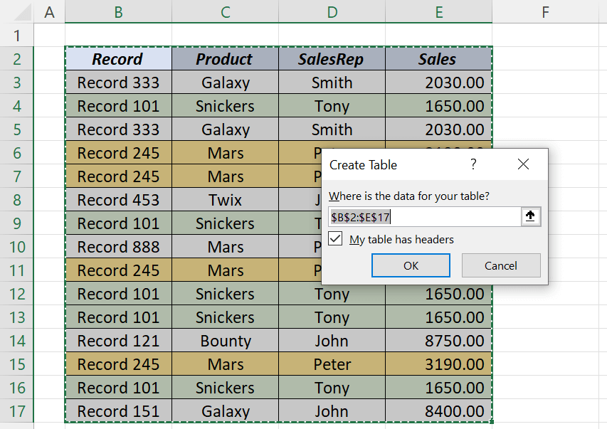
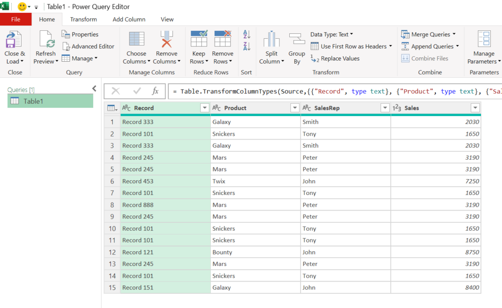
Click on OK in the Create Table dialog and the selected data will be loaded into the Power Query Editor of Excel.
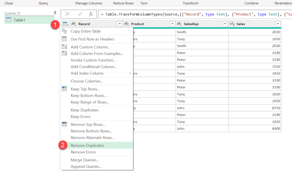
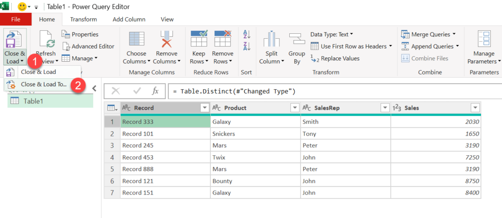
To remove duplicates, click on the icon in the top left corner of the work area and select Remove Duplicates from the list of options.
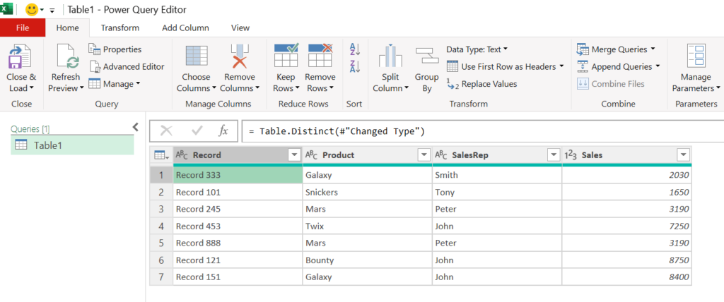
Duplicate records are all gone!
Now, to load this data into the Excel Worksheet,
Click on Close & Load in the Home tab of the Power Query Editor > Close Load To…
Import Data dialog is activated.
In this dialog we have to specify the location where we want to insert the data cleaned using Power Query. Here, I have selected the cell G2.
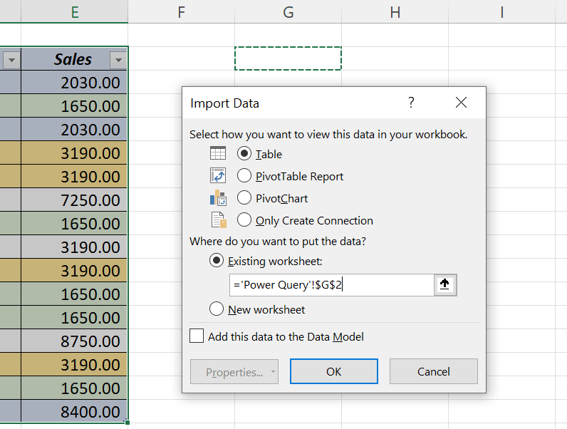
Click on OK and the data from Power Query Editor will be inserted into the specified cell.
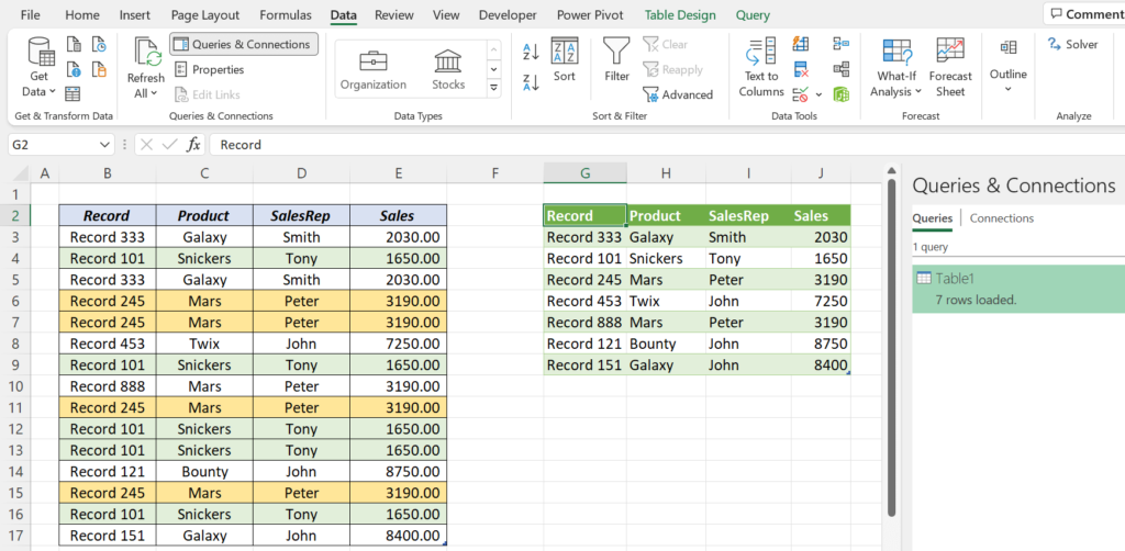
Unlike majority of the methods explained here, this method for removing duplicates using Power Query is a dynamic one.
The output table can updated for ‘Addition’ or ‘Deletion’ of data with a single click on the ‘Refresh‘ button in the Data tab of the Excel ribbon.
Pivot Table to remove duplicates
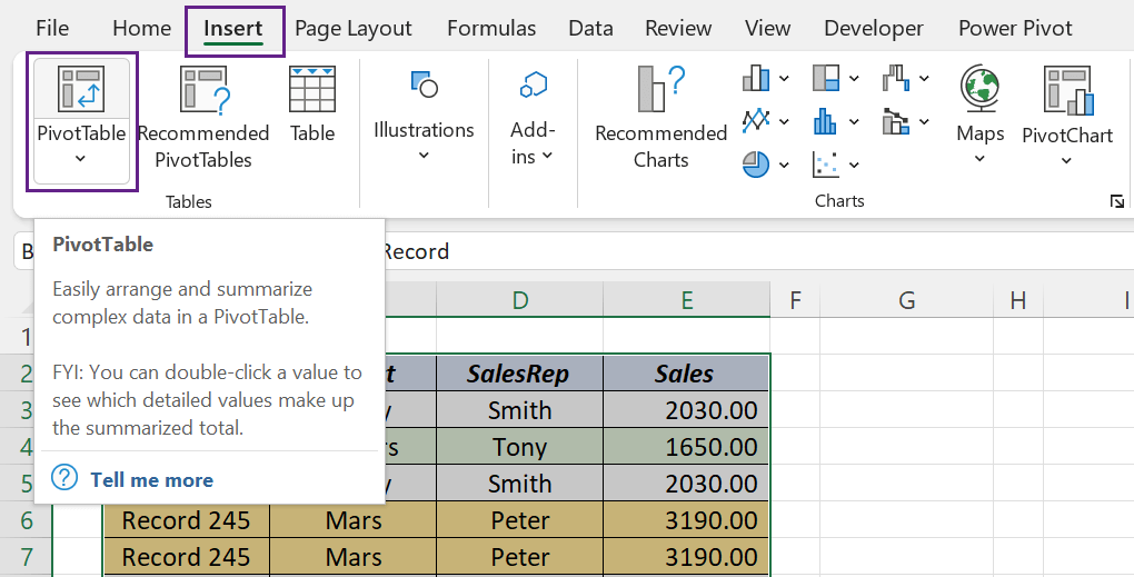
PivotTable in Excel also can be used when you want to create the unique list of values from a column.
Suppose we want to create the list of Sales representatives from the source data.
Select the cells containing data > go to the Insert tab of the Excel ribbon > click on PivotTable
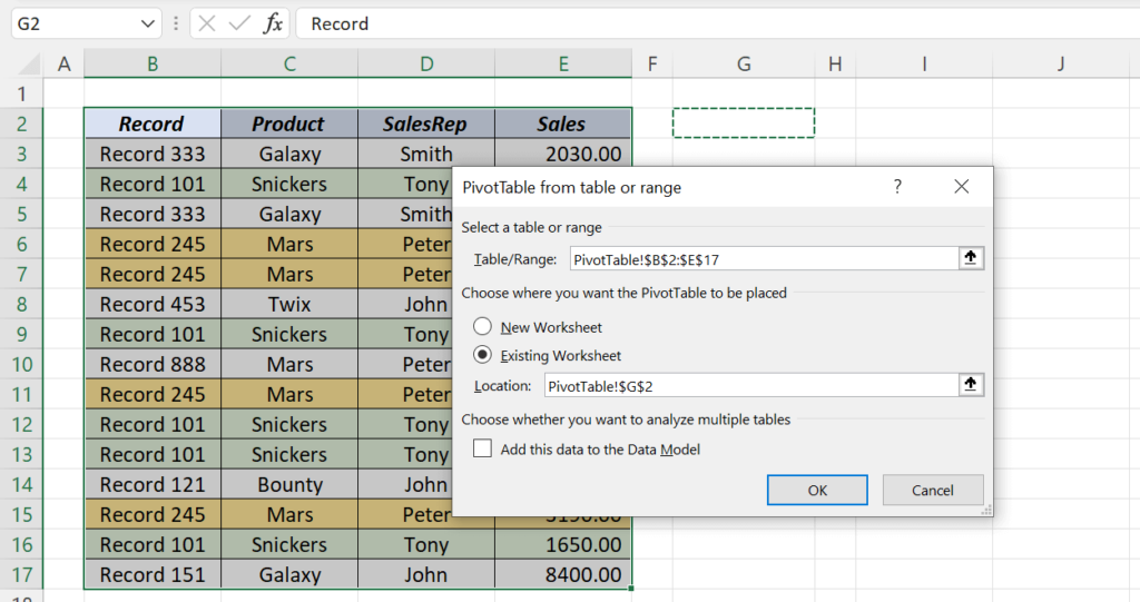
A dialog called PivotTable from table or range will be activated.
Use this dialog to specify the location where you want to insert the PivotTable. In this case, I want the Pivot Table in the cell G2 of the same sheet.
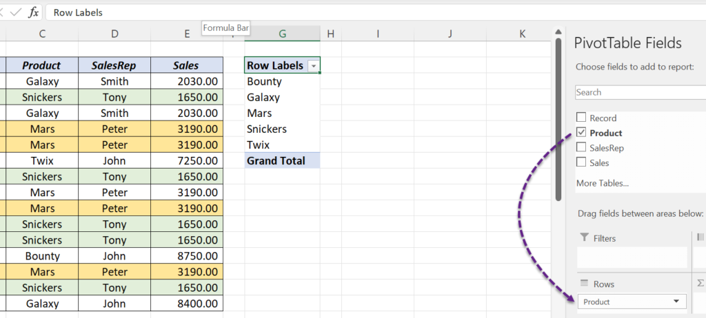
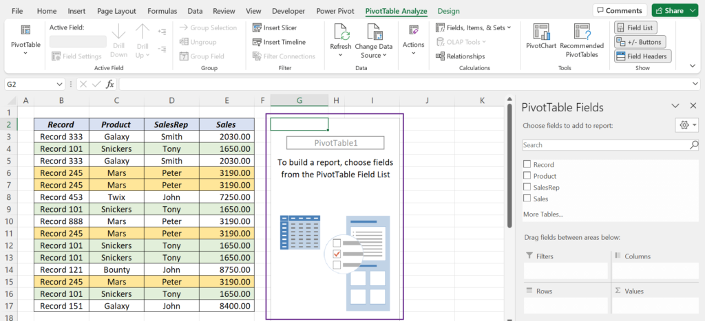
A PivotTable placeholder is created in the cell G2.
Drag and drop the PivotTable Field called SalesRep into the area for Rows and the PivotTable will display the unique list of Sales reps.
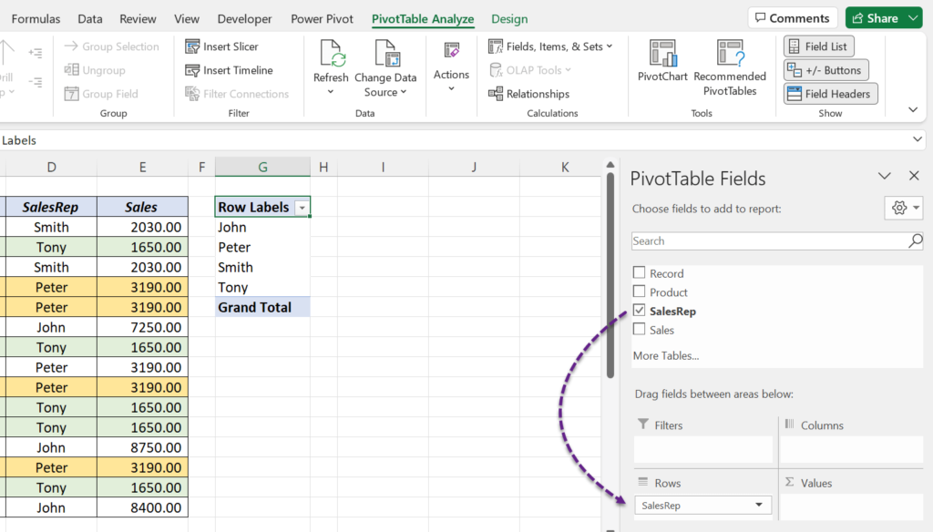
For the unique list of products, use the PivotTable field, Product.